Chapter 2 Basic data wrangling
2.1 What is data wrangling?
Data wrangling involves the manipulation of data into a form that is ready for visualisation. Typical steps in data wrangling often include (i) extracting the raw data and reading it into R, (ii) cleaning the data by handling missing values and outliers if any and (iii) summarising or transforming the data appropriately.
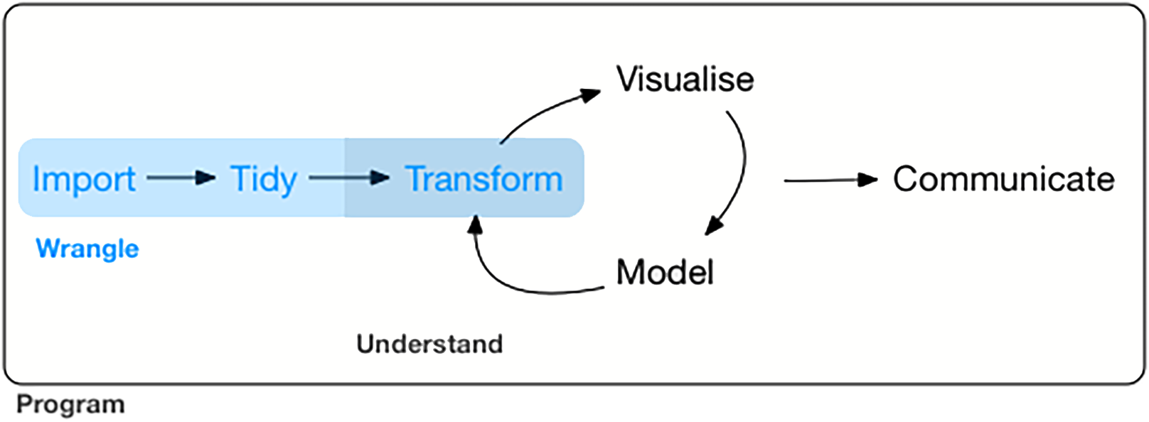
Figure 2.1: Data wrangling (marked blue) in the grand scheme of visualisation and modelling. Image taken from https://bookdown.org/roy_schumacher/r4ds/wrangle-intro.html
There is a collection of R packages for data science, collectively known as
the tidyverse. This includes the dplyr and ggplot2 package which we will
be using for data wrangling and visualisation respectively.
2.2 dplyr: grammar of data manipulation
The dplyr package provides a grammar for data manipulation, providing a
consistent set of verbs (i.e. operations / actions) that help to solve common
data manipulation challenges. These verbs include:
arrange()changes the ordering of the rows
select()picks variables based on their names
filter()picks cases based on their values
mutate()adds new variables that are functions of existing variables
summarise()reduces multiple values down to a single summary
There are also several other useful functions, namely:
pivot_wider()to change data from long to wide formatpivot_longer()to change data from wide to long formatgroup_by()allows one to perform operation “by group”inner_join()to join two datasets
To get a better understanding of these verbs and functions, we are going to apply them to data in the subsequent subsections and observe how the data changes.
2.2.1 Converting between long and wide formats
To illustrate how the data changes under different operations, we will use a small dataframe containing some values taken from four different years (2017-2020, represented in rows) and three different countries (sgp, jpn, aus, represented in columns). This matrix-like format is called the wide format where the data is distributed both vertically and horizontally. Wide format data are often more intuitive to humans as data across two attributes (corresponding to the rows and columns) can be represented succintly.
library(tidyverse)
df_wide = data.frame(
  year = c(2017,2018,2019,2020),
  sgp = c(100,120,140,160),
  jpn = c(550,575,600,650),
  aus = c(300,350,400,450))
df_wide
## year sgp jpn aus
## 1 2017 100 550 300
## 2 2018 120 575 350
## 3 2019 140 600 400
## 4 2020 160 650 450Here, we are going to convert the data from a wide format to a long format.
Long format data are list-like where the data spans vertically down the list.
This is preferred in data science since each row is a single data point and
the columns represents either some attribute (in this case, year/country)
or the data itself (value column). Thus, data points can be easily filtered
or manipulated based on the attributes, which we will see examples of later.
To convert the data from wide to long, we use the pivot_longer() function.
The !year argument specifies not to pivot the year column, keeping it as
the first attribute. The names_to = "country" specifies the column name for
the horizontal axis, in this case the country attribute. The
values_to = "value" specifies the column name for the data itself, which are
the numbers.
Note that we will be constantly using the %>% pipe operator here, which
“connects” the dataframe to the function. Multiple %>% can then be used to
apply multiple functions consecutively. In this example, we added an additonal
arrange(desc(country)), which arranges the long format data in descending
order according to the country.
df1 = df_wide %>%
  pivot_longer(!year, names_to = "country", values_to = "value") %>%
  arrange(desc(country))
df1
## # A tibble: 12 x 3
## year country value
## <dbl> <chr> <dbl>
## 1 2017 sgp 100
## 2 2018 sgp 120
## 3 2019 sgp 140
## 4 2020 sgp 160
## 5 2017 jpn 550
## 6 2018 jpn 575
## 7 2019 jpn 600
## 8 2020 jpn 650
## 9 2017 aus 300
## 10 2018 aus 350
## 11 2019 aus 400
## 12 2020 aus 450To convert long data into wide format, one can use the pivot_wider()
function, specifying the horizontal axis via names_from = "country" and the
column to populate the data via values_from = "value".
## # A tibble: 4 x 4
##    year   sgp   jpn   aus
##   <dbl> <dbl> <dbl> <dbl>
## 1  2017   100   550   300
## 2  2018   120   575   350
## 3  2019   140   600   400
## 4  2020   160   650   450
2.2.2 Subsetting data
A common task in data wrangling is to select a subset of the data based on
some attribute of the data. This can be achieved by the filter() function
and specifying the condition as the argument. In this example, we filter data
related to the sgp country by specifying country == "sgp". == is the
logical operator for “exactly equals to”. All other logical operators can also
be used such as not equals !=, contains %in%, more than or equal >= and
less than or equal <=. These logical operators can also be combined using
the AND logic & as well as the OR logic |.
## # A tibble: 4 x 3
##    year country value
##   <dbl> <chr>   <dbl>
## 1  2017 sgp       100
## 2  2018 sgp       120
## 3  2019 sgp       140
## 4  2020 sgp       160
Another way to subset the data is to select certain columns in the data. This
is mainly to declutter the data and remove any unnecessary information. This
is performed using the select() function and specifying the columns to keep.
Here, we combined both the filtering step above and selecting for only the
year and value column since the country information is no longer necessary.
## # A tibble: 4 x 2
##    year value
##   <dbl> <dbl>
## 1  2017   100
## 2  2018   120
## 3  2019   140
## 4  2020   160
2.2.3 Transforming data
Apart from subsetting data, one might want to transform the data to suit
analysis needs. This can be done using the mutate() function which adds a
new column of values that are functions of existing columns. The function is
applied row-wise in a one-to-one manner i.e. each row will have a new value,
making up a new column. In the example below, we did logval = log10(value),
which creates a new column logval calculated as the log10 of the value
column. The mutate() function is very versatile: (i) more complicated tasks
like replacing text is possible and (ii) mutate can be applied on selected
rows based on some condition.
## # A tibble: 12 x 4
##     year country value logval
##    <dbl> <chr>   <dbl>  <dbl>
##  1  2017 sgp       100   2
##  2  2018 sgp       120   2.08
##  3  2019 sgp       140   2.15
##  4  2020 sgp       160   2.20
##  5  2017 jpn       550   2.74
##  6  2018 jpn       575   2.76
##  7  2019 jpn       600   2.78
##  8  2020 jpn       650   2.81
##  9  2017 aus       300   2.48
## 10  2018 aus       350   2.54
## 11  2019 aus       400   2.60
## 12  2020 aus       450   2.65
Another way to transform the data is to summarise the data, i.e. reduce
multiple values to a single summary. Functions are applied in a multi-to-one
manner i.e. multiple values are combined such as the sum or mean. We also
seperate the data into groups and obtain summaries for each of the groups.
Indeed, in the example below, we first group the data by country using
group_by(country) and then calulated the sum for each country using
summarise(total = sum(value)). Notice that the output only contains the
country column (i.e. the column you group by) and total column (i.e. the
summary).
## `summarise()` ungrouping output (override with `.groups` argument)## # A tibble: 3 x 2
## country total
## <chr> <dbl>
## 1 aus 1500
## 2 jpn 2375
## 3 sgp 5202.2.4 Joining data
Another common task in data wrangling is to join two different datasets.
Different information / attributes are often stored in different datasets as
such compartmentalization rersults in smaller storage space. For example, here
we introduce another dataframe dfAdd containing the information on which
region each country belong to.
##   country  region
## 1     sgp    asia
## 2     jpn    asia
## 3     aus oceania
We can then join the previous year, country, value dataframe with this new
dataframe to include regional information. This is performed using the
inner_join(), specifying the new dataframe dfAdd and providing a key
column by = "country" to do the join. This now gives us greater flexibility
to perform data manipulation based the region. Note that there are other join
functions as well, such as left_join() and outer_join(), which retains
different parts of the data.
## # A tibble: 12 x 4
##     year country value region
##    <dbl> <chr>   <dbl> <fct>
##  1  2017 sgp       100 asia
##  2  2018 sgp       120 asia
##  3  2019 sgp       140 asia
##  4  2020 sgp       160 asia
##  5  2017 jpn       550 asia
##  6  2018 jpn       575 asia
##  7  2019 jpn       600 asia
##  8  2020 jpn       650 asia
##  9  2017 aus       300 oceania
## 10  2018 aus       350 oceania
## 11  2019 aus       400 oceania
## 12  2020 aus       450 oceania
2.3 Data wrangling on COVID-19 statistics
Now, we can apply the dplyr verbs and functions that we learnt in dechiphering
COVID-19 statistics, namely the number of confirmed / recovered / deaths in
each country on each day. To retrieve this data, we can use the coronavirus
R package, which can be installed via install.packages("coronavirus").
2.3.1 Initial inspection of data
Before data wrangling, it is important to first get a “feel” of the data
through some initial inspection. The COVID-19 statistics is first loaded via
dfmain = coronavirus and the first few rows were outputted head(dfmain).
We then ran the summary() function on columns containing continuous values
and checked the first few unique entries for columns containing text. Notably,
the data in in a long format and the type column informs whether the number
of cases in cases are referring to confirmed / recovered / deaths.
##         date province     country      lat     long      type cases
## 1 2020-01-22          Afghanistan 33.93911 67.70995 confirmed     0
## 2 2020-01-23          Afghanistan 33.93911 67.70995 confirmed     0
## 3 2020-01-24          Afghanistan 33.93911 67.70995 confirmed     0
## 4 2020-01-25          Afghanistan 33.93911 67.70995 confirmed     0
## 5 2020-01-26          Afghanistan 33.93911 67.70995 confirmed     0
## 6 2020-01-27 Afghanistan 33.93911 67.70995 confirmed 0## Min. 1st Qu. Median Mean 3rd Qu.
## "2020-01-22" "2020-03-21" "2020-05-19" "2020-05-19" "2020-07-17"
## Max.
## "2020-09-14"## [1] "" "Alberta"
## [3] "Anguilla" "Anhui"
## [5] "Aruba" "Australian Capital Territory"
## [7] "Beijing" "Bermuda"
## [9] "Bonaire, Sint Eustatius and Saba" "British Columbia"## [1] "Afghanistan" "Albania" "Algeria"
## [4] "Andorra" "Angola" "Antigua and Barbuda"
## [7] "Argentina" "Armenia" "Austria"
## [10] "Azerbaijan"## [1] "confirmed" "death" "recovered"## Min. 1st Qu. Median Mean 3rd Qu. Max.
## -16298.0 0.0 0.0 268.2 8.0 140050.02.3.2 No. confirmed cases in Singapore as of 1st Sep 2020
Let us do an example to determine the total number of confirmed COVID-19 cases
in Singapore as of 1st Sep 2020. Clearly, we are interested in (i) Singapore,
(ii) confirmed cases and (iii) cases as of 1st Sep 2020. Thus, we filter the
data based on these three criterion. We then sum up the cases to give us the
total number via summarise(totalcases = sum(cases)).
dfmain %>%
  filter(country == "Singapore") %>%
  filter(type == "confirmed") %>%
  filter(date <= "2020-09-01") %>%
  summarise(totalcases = sum(cases))
## totalcases
## 1 568522.3.3 Top 10 countries (confirmed cases) as of 1st Sep 2020
Next, let us determine the top 10 countries in terms of total number of confirmed COVID-19 cases. To increase the challenge, we would also want to know the total number of recovered and deaths as well as the proportion of active cases i.e. confirmed - death - recovered.
To do this, we first do filter(date <= "2020-09-01") to ensure that we are
in the correct timeframe. Next, we want to calculate the total number of
confirmed / recovered / deaths separately for each individual country. This
requires us to group the data by both country and type
group_by(country, type), followed by summing the cases
summarise(totalcases = sum(cases)). Next, in order to calculate the
proportion of active cases, we need to have the confirmed / recovered / deaths
in different columns, which we achieve by converting the data into a wide
format pivot_wider(names_from = type, values_from = totalcases). Then, we
can proceed to calculate the proportion of active cases
mutate(propActive = round((confirmed-death-recovered) / confirmed, 3)).
Finally, the countries are arranged in descreasing order by confirmed cases
and the top 10 countries are then displayed.
dfmain %>%
  filter(date <= "2020-09-01") %>%
  group_by(country, type) %>%
  summarise(totalcases = sum(cases)) %>%
  pivot_wider(names_from = type, values_from = totalcases) %>%
  mutate(propActive = round((confirmed-death-recovered) / confirmed, 3)) %>%
  arrange(desc(confirmed)) %>%
  head(10)
## # A tibble: 10 x 5
## # Groups: country [10]
## country confirmed death recovered propActive
## <chr> <int> <int> <int> <dbl>
## 1 US 6073840 184664 2202663 0.607
## 2 Brazil 3950931 122596 3345240 0.122
## 3 India 3769523 66333 2901908 0.213
## 4 Russia 997072 17250 813603 0.167
## 5 Peru 652037 28944 471599 0.232
## 6 South Africa 628259 14263 549993 0.102
## 7 Colombia 624026 20050 469552 0.215
## 8 Mexico 606036 65241 501722 0.064
## 9 Spain 470973 29152 150376 0.619
## 10 Argentina 428239 8919 308376 0.259