Chapter 5 More Dimension Reduction

5.1 Why perform dimension reduction?

Single-cell data, such as scRNA-seq, typically includes thousands of genes (features) for each cell (sample). This results in high-dimensional data that can be challenging to interpret and analyze directly. Reducing dimensions simplifies the dataset, making it more manageable. Furthermore, working with reduced dimensions decreases the computational burden, making downstream analyses faster and more efficient. Thus, dimension reduction is performed prior to many downstream analysis such as cell clustering (Section 3) and trajectory inference analysis (Section 6). Here, we will further discuss the rationale behind performing dimension reduction. We will also examine certain considerations when interpreting the fidelity of dimension reduction methods.

There are several reasons for performing dimension reduction (Figure 5.1). First, by reducing the data to 2D or 3D, one can easily visualize and interpret the data. This is especially important for human interpretation to observe patterns, clusters, and relationships between cells as we are not used to perceiving the world beyond 3D. Visual inspection of the data allows us to identify general cell populations and check if cells are grouping by any technical factors i.e. nUMI and pctMT or batch effect. This can also help in making the biological interpretation more straightforward, allowing researchers to focus on the most significant patterns and relationships in the data. Second, dimension reduction reduces the random noise in the data. High-dimensional scRNA-seq data often includes noise, which can obscure the biological signal. Dimension reduction techniques, like PCA, can help filter out this noise by focusing on the components that capture the most variance, thereby enhancing the signal-to-noise ratio. The noise often manifest as higher dimensions and these higher dimensions can be discarded to better distinguish any biological signal in downstream analysis. In fact, deep learning models such as autoencoders utilizes such concepts where the data is compressed / encoded from high to low dimensions and then decoded back to the original state. This encode-decode process “squeezes” out the random noise, ensuring that only meaningful signal is retained. Third, dimension reduction avoids the curse of dimensionality (Altman and Krzywinski 2018). As the number of dimension increases, the “volume” that data can occupy increases rapidly. This resulting data becomes very sparse, making it difficult to identify differences between data points as the distances between samples becomes very similar. Furthermore, as the number of dimensions increases, many of these dimensions tend to be related to each other. Some of the downstream analysis may have problems dealing with this multicollinearity. In fact, this is common in biology where many genes (which are the features / dimensions) often act in a concerted manner during some biological process. Thus, dimension reduction seeks to “consolidate” these related dimensions and summarise them.

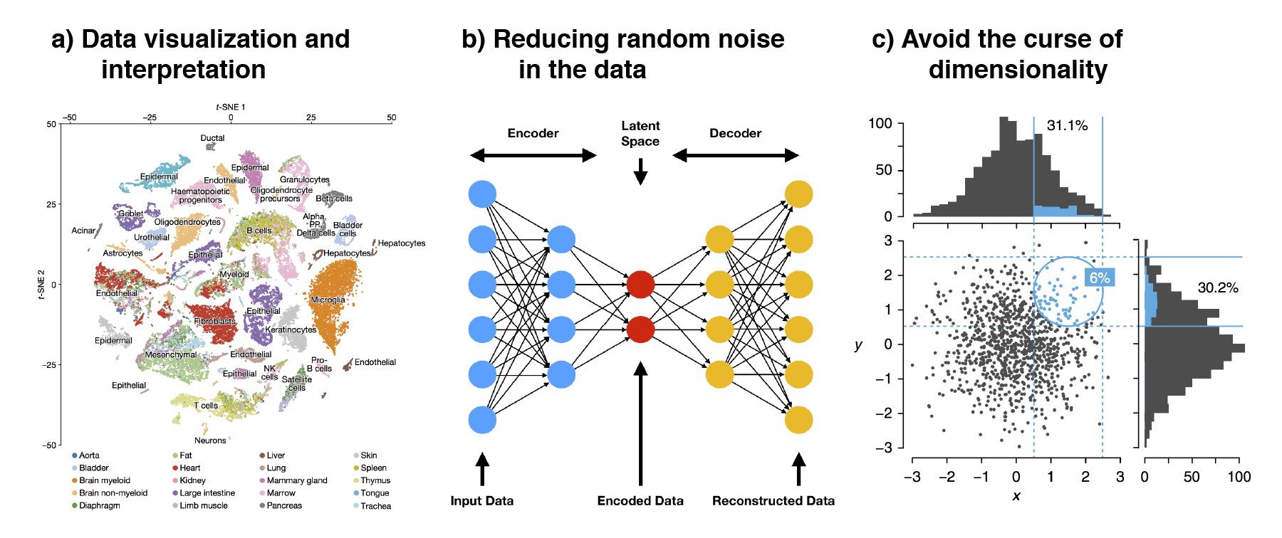
Figure 5.1: The three main reasons to perform dimension reduction in single-cell analysis is for (a) data visualization, (b) removal of random noise by “discarding” higher dimensions and (c) to avoid the curse of dimensionality.

5.2 Local and global structure in DR

In dimension reduction, local and global structure refer to the different aspects of the data that are preserved or emphasized during the reduction process. These structures are crucial when choosing a dimension reduction method, depending on what aspects of the data are most important to your analysis (Figure 5.2).

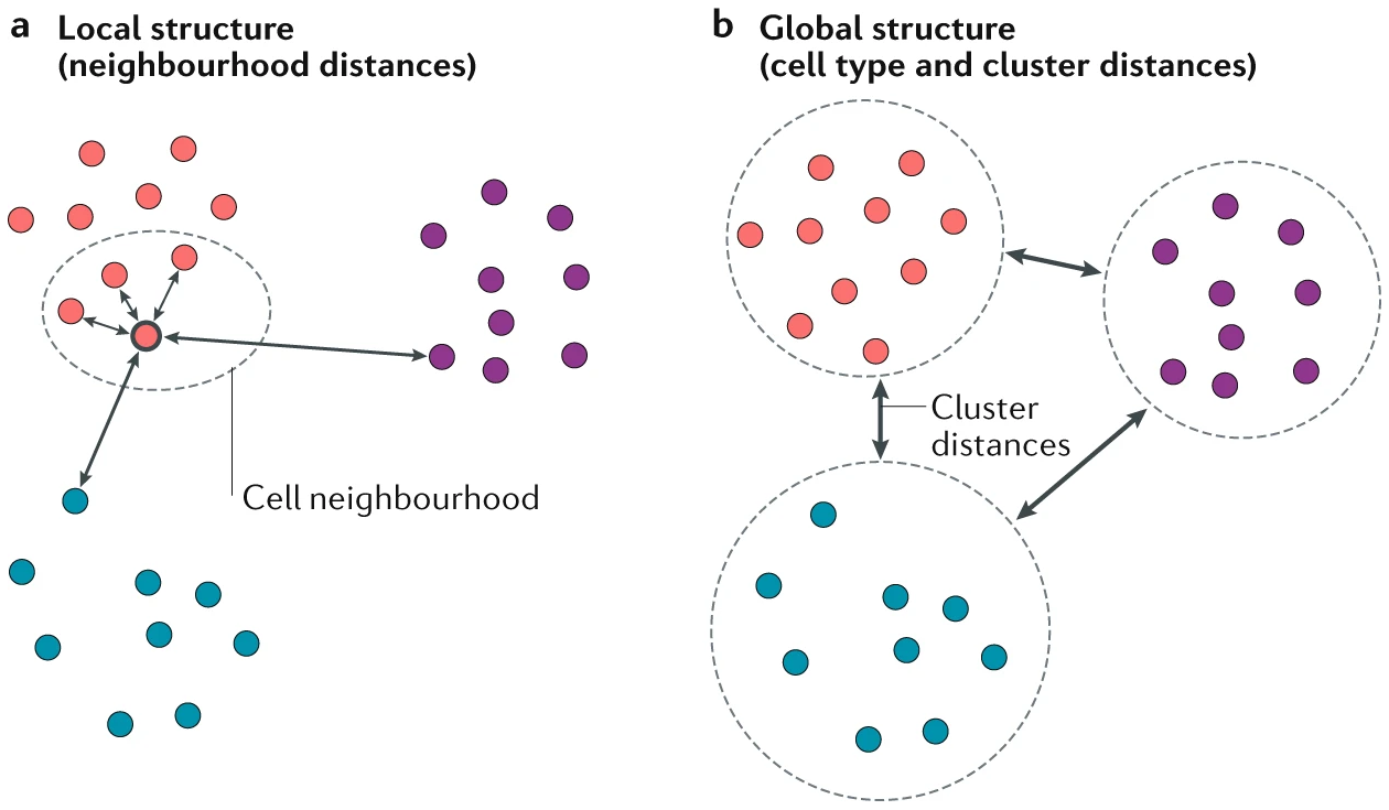
Figure 5.2: (a) Preserving the local structure of a dataset ensures that the neighbouring cells of each cell remain together in the visualization, rather than preserving the original gene expression space. The distance between cells in the final visualization is therefore representative of the degree of similarity between their gene expression patterns. (b) Preserving the global structure of a dataset ensures that large-scale distances, such as the distances between cell types, are maintained. Image taken from https://www.nature.com/articles/s41581-020-0262-0

Local structure refers to the relationships between transcriptionally similar single cells in the high-dimensional gene expression space. This includes the preservation of small distances and the local neighborhood of points, meaning that points that are close together in high-dimensional space should remain close in the reduced-dimensional space. Preserving local structure is particularly useful in tasks such as identifying local clusters, analyzing subpopulations, or detecting small-scale patterns within the data. t-SNE is an example dimension reduction technique that emphasizes local structure by maintaining the relative distances between close points. Thus, t-SNE reductions often clump transcriptionally similar cells into distinct clusters, which is suitable for cell type identification in atlasing projects.

Global structure refers to the broader, overall relationships and patterns in the data, such as large-scale distances between distant points, the general shape or geometry of the data distribution, and the relationships between different clusters or cell populations in the data. Preserving global structure is important when the focus is on understanding the overall relationships between cell populations, which is also an end goal of trajectory inference analysis. Thus, it is crucial to apply trajectory inference on reduced dimensions that preserve global structure well. Some algorithms, such as PCA, excels at preserving global structure, as PCA rotates the data without any distortion and maximises the variance captured (which is essentially the global structure) in the top principal components. Other algorithms such as UMAP and force-directed layout (FDL) aims to balance between preserving both global and local structure. In biological systems where a continuum of cell state is expected e.g. bone marrow, development and differentiation timeseries, reductions that preserve global structure should visually appear “flowly”, joining early-to-late or progenitor-to-differentiated populations.

5.3 Varying UMAP parameters

UMAP (Uniform Manifold Approximation and Projection) is designed to preserve both local and global structures of the data, thus making it popular for visualizing high-dimensional single-cell data. UMAP works by constructing a high-dimensional graph representation of the data, where each data point is connected to its nearest neighbors based on their similarity. This graph is then projected into a lower-dimensional space, typically 2D or 3D, while trying to maintain the structure of the original graph as much as possible (Figure 5.3). The algorithm optimizes the layout by minimizing the difference between the high-dimensional graph and its low-dimensional counterpart.

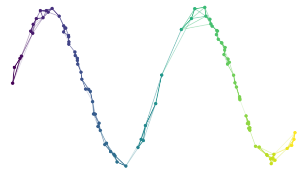
Figure 5.3: In UMAP, a graph representation of the input high-dimensional data is created and then projected into a lower-dimensional space while trying to maintain the structure of the original graph. Image taken from https://umap-learn.readthedocs.io/en/latest/how_umap_works.html

UMAP’s performance and the nature of the resulting reductions are strongly influenced by two main parameters: n_neighbors and min_dist. First, the n_neighbors parameter controls the size of the local neighborhood used when constructing the high-dimensional graph. It determines how many of the closest points (neighbors) around each data point are considered when defining its local structure. Smaller n_neighbors (e.g., 5-15) emphasizes local structure and can lead to a more fragmented / clumpy embedding, where small clusters of similar points are tightly packed together. Larger n_neighbors (e.g., 50-100) emphasizes global structure, resulting in a more connected / flowly embedding that reflects larger patterns and relationships across the entire dataset.

Second, the min_dist parameter controls the minimum distance between points in the low-dimensional space. It effectively governs how tightly UMAP packs the points together in the embedding. Smaller min_dist (e.g., 0.1) leads to a more compact embedding, resulting in tight clusters and can highlight distinct groupings or very close relationships within the data. Larger min_dist (e.g., 0.5) results in a more spread-out embedding, allowing for a clearer distinction between different groups or clusters in the data.

In the bone marrow example (Figure 5.4), we do observe the data points becoming more spread out as the min_dist is increased. Also, there are slight changes in the relationship between CMP, EOBM and ERP as n_neighbors is being increased.

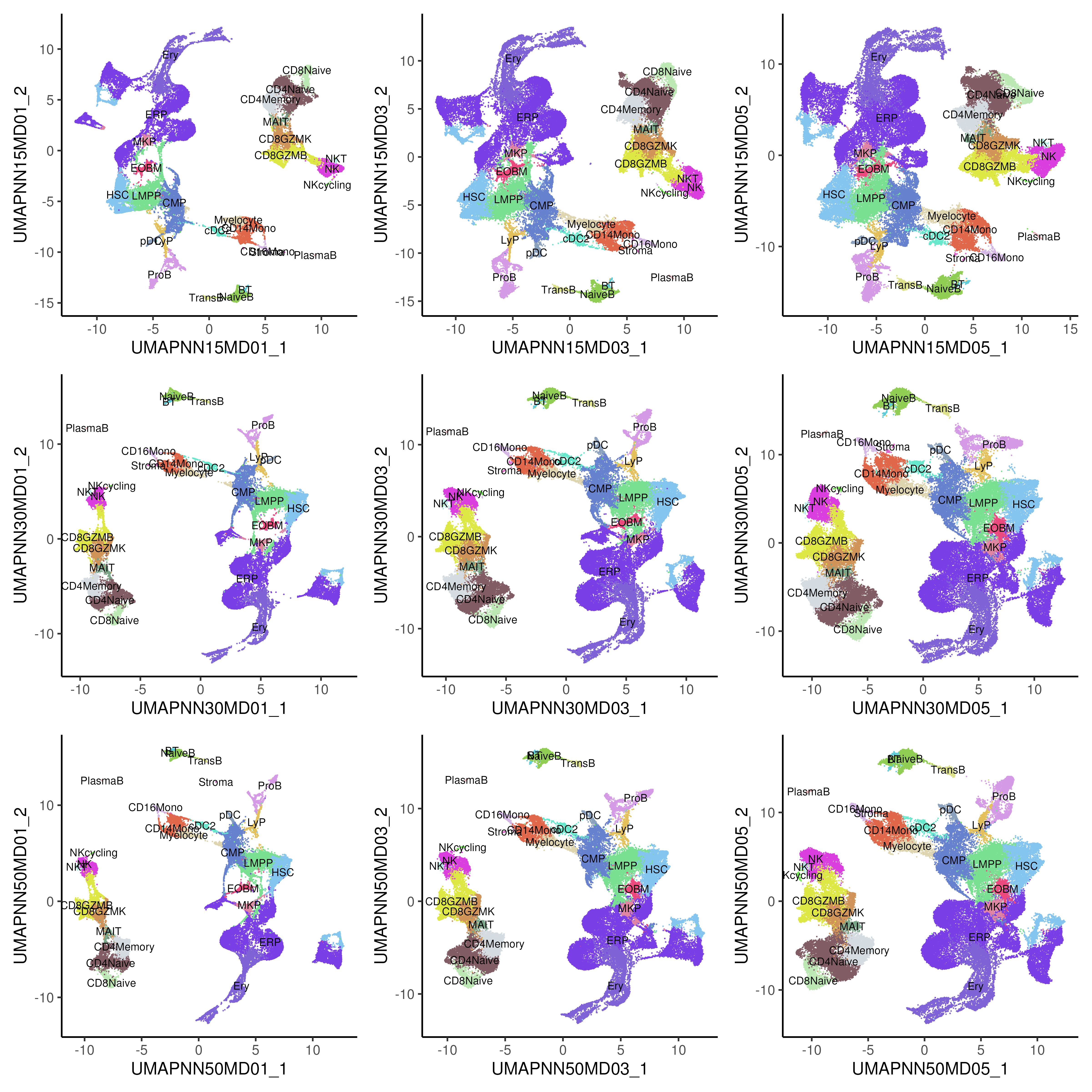
Figure 5.4: UMAP of healthy and CML bone marrow, generated using varying parameters of number of n_neighbors (NN) and min_dist (MD). Top / middle / bottom row uses 15 / 30 / 50 NN correspondingly while left / middle / right column uses 0.1 / 0.3 / 0.5 MD correspondingly.

5.4 Force-directed layout

Force-Directed Layout (FDL) algorithms are a class of techniques used for graph visualization, where data points (nodes) are positioned in a space such that their layout reflects the underlying structure of the graph. These algorithms simulate physical systems where forces, such as attraction and repulsion, act between the points / nodes, leading to an arrangement that reveals clusters, trajectories, or other relationships within the data.

The ForceAtlas2 (FA2) algorithm is a popular and enhanced version of an FDL algorithm. It’s widely used in graph analysis, particularly in the visualization of large networks like social graphs or single-cell network graphs. Briefly, the ForceAtlas2 algorithm models the graph as a physical system where points / nodes are represented as particles that exert forces on each other. The edges, representing connections between nodes, act like springs that pull connected nodes closer together. These edges are usually constrcuted for the k-nearest neighbours for each point.

FDL algorithms are useful for trajectory analysis in single-cell studies. Such trajectory analysis involves understanding the progression or differentiation of cells through different states or stages. These trajectories can be thought of as paths within a graph, where each node represents a cell, and edges represent transitions or similarities between states. The spring-like attractive forces between connected nodes ensure that cells with similar states or those in close stages of differentiation are positioned near each other. This helps in clearly visualizing the continuous progression of cell states along a trajectory.

In the bone marrow example (Figure 5.5), we do observe a more continuous progression from progenitor cells to differentiated cells between the different lineages in the bone marrow e.g. myeloid, erythroid and B-lymphoid linages.

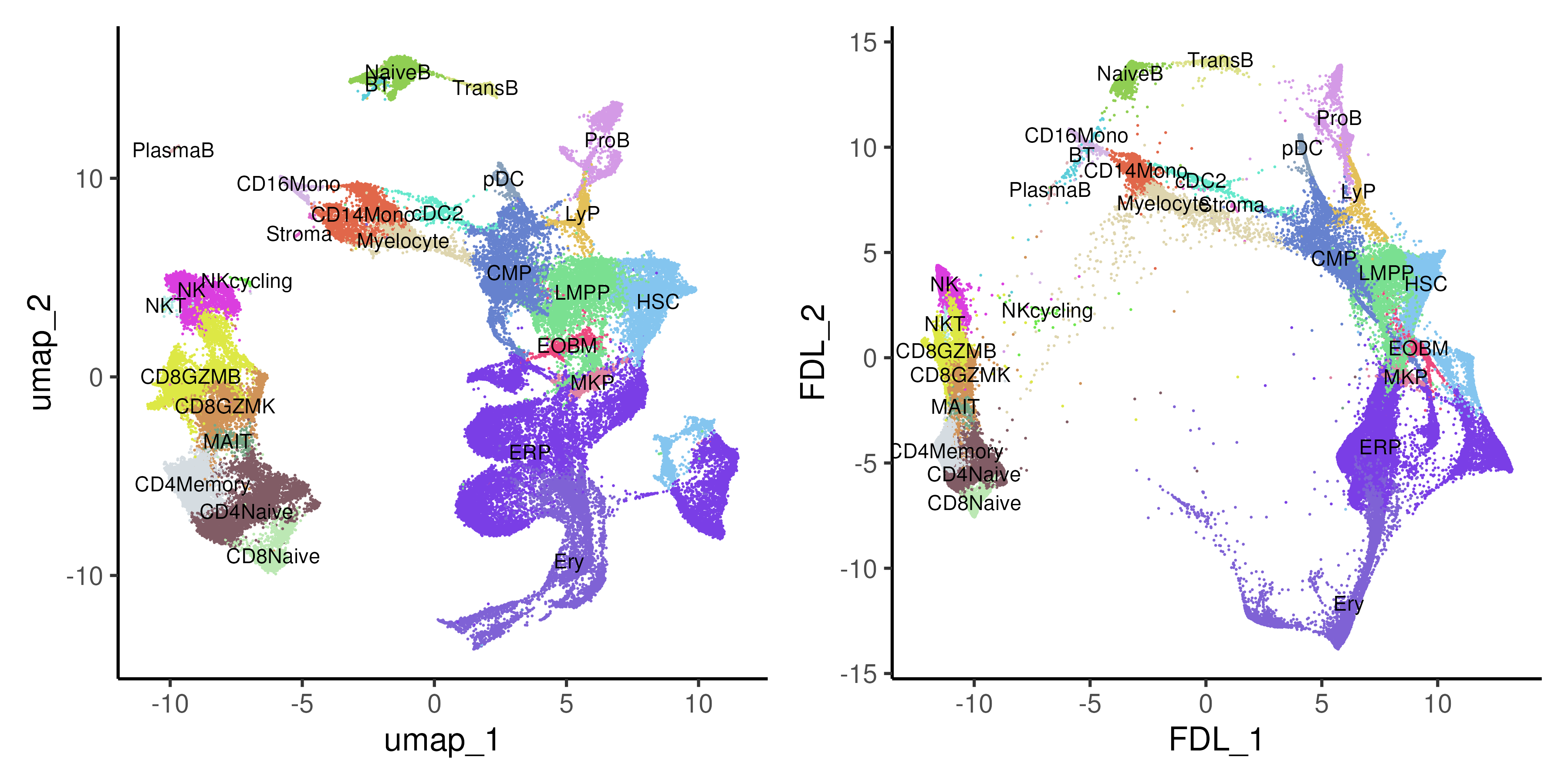
Figure 5.5: UMAP and force-directed layout (FDL) of healthy and CML bone marrow data coloured by annotated cell types.

5.5 Diffusion maps

Diffusion Maps are a non-linear dimension reduction technique that is useful in single-cell analysis for capturing the underlying structure of complex datasets, such as continuous processes and trajectories. Diffusion Maps model the data as a random walk on a graph, where each point / single cell is a node, and edges represent the similarity between nodes. The key idea is to simulate the diffusion process on this graph, where the probability of moving from one node to another depends on their similarity. The algorithm then uses the diffusion process to determine the “diffusion distance” between points, which is then reduce the data to a lower-dimensional space that preserves the intrinsic geometry of the data, particularly the relationships that are most important for understanding the underlying biological processes.

Due to the diffusion nature of the method, diffusion maps excel at preserving the continuity of cell states, which is crucial for understanding continuous biological processes like cell differentiation. In cases where cells diverge into different fates (e.g., stem cells differentiating into multiple cell types), diffusion maps can help identify these branching points and the paths leading to different outcomes. However, diffusion maps do have disadvantages. Diffusion maps often generate more than two components to capture the underlying structure of the data, making visualization and interpretation more challenging. Unlike PCA, where the first two components often capture the majority of the variance, in diffusion maps, important information might be spread across multiple components. This means that the user needs to carefully consider which components to examine, potentially requiring the visualization of 3D plots or multiple 2D plots covering different diffusion components.

In the bone marrow example (Figure 5.6), we visualized the top five diffusion components and found that different components describe different major sources of biological variation in the system especially celltype differences. For example, DC_2 is separating the myeloid / erythroid lineages while DC_3 is describing the variation across the B-cell celltypes.

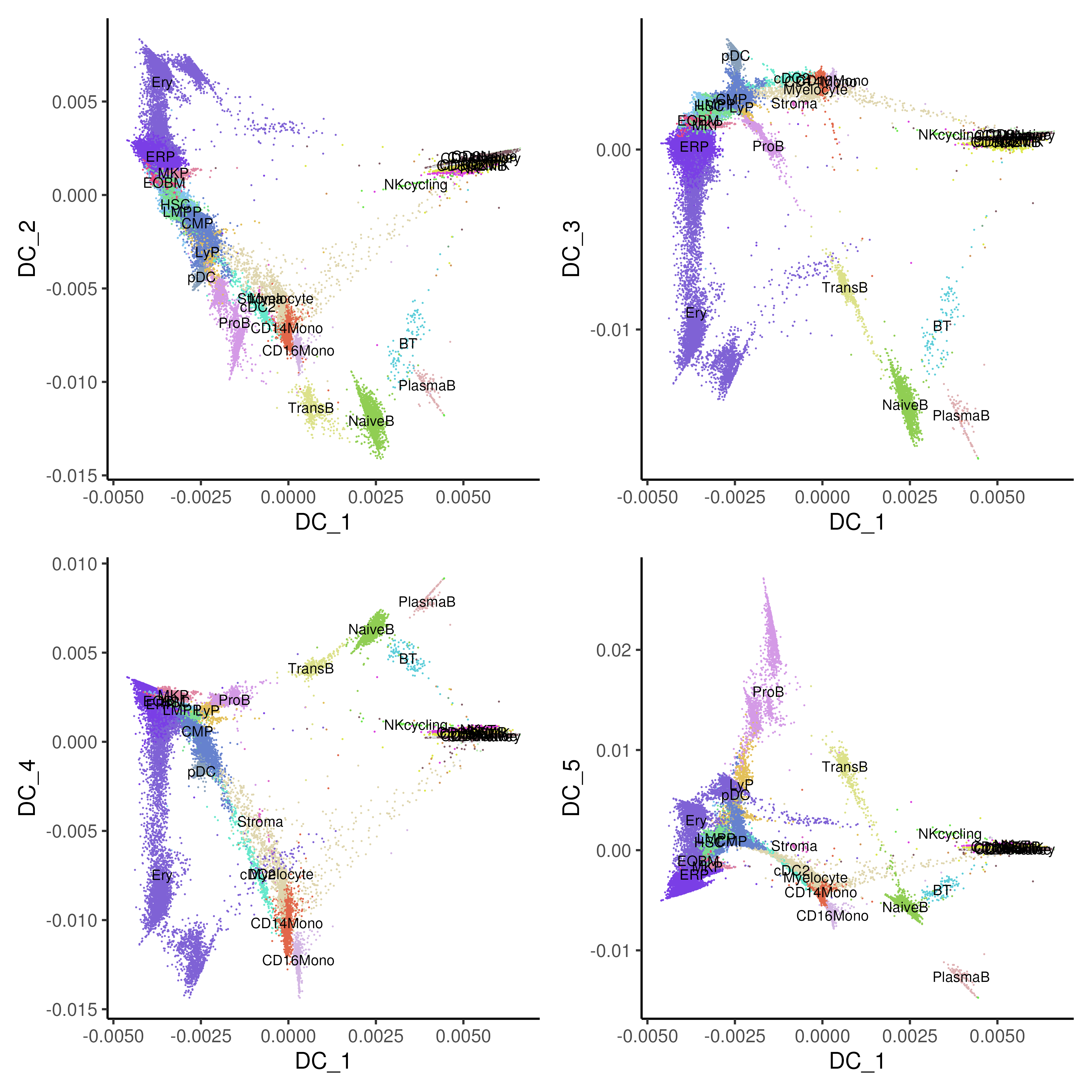
Figure 5.6: Diffusion maps with component 1 on x-axis and component 2-5 on y-axis of healthy and CML bone marrow data coloured by annotated cell types.

5.6 PHATE

PHATE (Potential of Heat-diffusion for Affinity-based Trajectory Embedding) is a dimension reduction and visualization method specifically designed for single-cell analysis (Figure 5.7). It excels at capturing and revealing both local and global structures in high-dimensional data, such as continuous trajectories and branching processes,. PHATE works by first constructing a diffusion map to capture the manifold structure of the data, and then applying a novel potential distance metric that preserves both fine details and broader trends. This results in a visually intuitive, low-dimensional embedding that highlights the trajectories and relationships between cells, even in noisy and complex datasets.

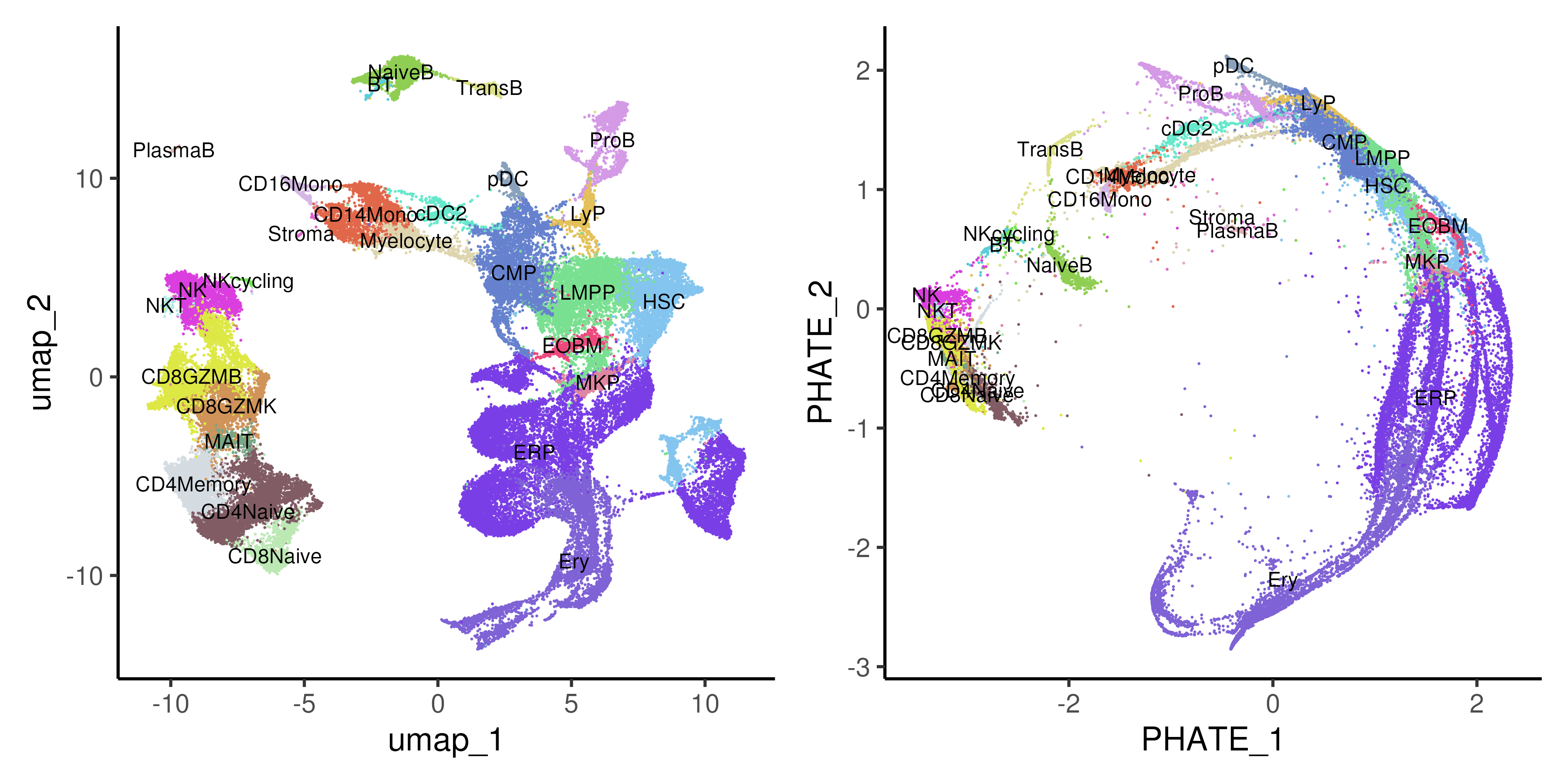
Figure 5.7: UMAP and Potential of Heat-diffusion for Affinity-based Trajectory Embedding (PHATE) of healthy and CML bone marrow data coloured by annotated cell types.

5.7 Code

##### Load required packages
rm(list = ls())
library(data.table)
library(Matrix)
library(ggplot2)
library(ggrepel)
library(patchwork)
library(randomcoloR)
library(RColorBrewer)
library(Seurat)
library(reticulate)
library(pdist)
library(phateR)
library(SeuratWrappers)
library(monocle3)
library(slingshot)
library(tradeSeq)
library(pheatmap)
library(clusterProfiler)
library(msigdbr)
library(BiocParallel)
if(!dir.exists("output/")){dir.create("output/")} # Folder to store outputs
use_python("/usr/bin/python3")    # py_config()
os <- import("os")
py_run_string("r.os.environ['OMP_NUM_THREADS'] = '4'")


### Define color palettes
colPat = brewer.pal(8, "Paired")                 # color for patients
names(colPat) = c("NBM250267","NBM40316","NBM80350","NBM90222",
                  "P677","P685","P735","P742")
colGEX = c("grey85", brewer.pal(9, "Reds"))      # color for gene expression
colCcy = c("black", "blue", "darkorange")        # color for cellcycle phase
set.seed(42); colCT  = distinctColorPalette(28)   # color for celltype



##### A. Varying UMAP parameters #####
seu <- readRDS("output/sec3_bmSeu.rds")
# vary both n.neighbors and min.dist
for(iNN in c(15,30,50)){
  for(iMD in c(0.1,0.3,0.5)){
    seu <- RunUMAP(seu, dims = 1:50, n.neighbors = iNN, min.dist = iMD,
                   reduction.name = paste0("UMAP_NN",iNN,"_MD",iMD))
  }
}
ggOut = list()
for(iNN in c(15,30,50)){
  for(iMD in c(0.1,0.3,0.5)){
    ggOut[[paste0("UMAP_NN",iNN,"_MD",iMD)]] <- 
      DimPlot(seu, reduction = paste0("UMAP_NN",iNN,"_MD",iMD), 
              pt.size = 0.1, label = TRUE, cols = colCT) + 
      theme_classic(base_size = 18) + NoLegend()
  }
}
ggsave(wrap_plots(ggOut), width = 16, height = 16, filename = "output/5A_varyUMAP.png")



##### B. Force-directed layout #####
# Setup python anndata for downstream DFL/DiffMap/PAGA
sc <- import("scanpy")
adata <- sc$AnnData(
  X   = np_array(t(GetAssayData(seu)[VariableFeatures(seu),]), dtype="float32"),
  obs = seu@meta.data[, c("patient", "celltype")],
  var = data.frame(geneName = VariableFeatures(seu)))
adata$obsm$update(X_pca = Embeddings(seu, "pca"))
adata$obsm$update(X_umap = Embeddings(seu, "umap"))
adata$var_names <- VariableFeatures(seu)
adata$obs_names <- colnames(seu)
sc$pp$neighbors(adata, n_neighbors = as.integer(30), n_pcs = as.integer(50))

# Tricks python to use modified version of fa2
py_run_string("import sys")
py_run_string("import fa2_modified")
py_run_string("sys.modules['fa2'] = fa2_modified")

# Calculate FDL
sc$tl$draw_graph(adata, layout = "fa", init_pos = "X_umap")
oupDR <- py_to_r(adata$obsm['X_draw_graph_fa'])
rownames(oupDR) <- colnames(seu)
colnames(oupDR) <- c("FDL_1","FDL_2")
oupDR = oupDR / 10^(floor(log10(diff(range(oupDR))))-1)
seu[["fdl"]] <- CreateDimReducObject(embeddings = oupDR, key = "FDL_",
                                     assay = DefaultAssay(seu))

# Plot FDL
p1 <- DimPlot(seu, reduction = "umap", pt.size = 0.1, label = TRUE, 
              cols = colCT) + theme_classic(base_size = 18) 
p2 <- DimPlot(seu, reduction = "fdl", pt.size = 0.1, label = TRUE, 
              cols = colCT) + theme_classic(base_size = 18)
ggsave(p1 + p2 & theme(legend.position = "none"), 
       width = 12, height = 6, filename = "output/5B_FDL.png")



##### C. DiffMaps #####
# Calculate DiffMaps
sc$tl$diffmap(adata)
oupDR <- py_to_r(adata$obsm['X_diffmap'])
rownames(oupDR) <- colnames(seu)
colnames(oupDR) <- paste0("DC_", 0:(15-1))
oupDR <- oupDR[, paste0("DC_", seq(10))]
seu[["diffmap"]] = CreateDimReducObject(embeddings = oupDR, key = "DC_",
                                        assay = DefaultAssay(seu))

# Plot DiffMaps
ggOut <- list()
for(i in 2:5){
  ggOut[[paste0("DC1",i)]] <- 
    DimPlot(seu, reduction = "diffmap", pt.size = 0.1, label = TRUE,
            cols = colCT, dims = c(1,i)) + theme_classic(base_size = 18)
}
ggsave(wrap_plots(ggOut) & theme(legend.position = "none"), 
       width = 12, height = 12, filename = "output/5C_diffMap.png")



##### D. PHATE #####
# Calculate PHATE
oupPhate = phate(t(GetAssayData(seu)[VariableFeatures(seu), ]), 
                 knn = 30, npca = 50, seed = 42)
oupDR = oupPhate$embedding
oupDR = oupDR / 10^(floor(log10(diff(range(oupDR)))))
rownames(oupDR) = colnames(seu)
colnames(oupDR) = c("PHATE_1","PHATE_2")
seu[["phate"]] <- CreateDimReducObject(embeddings = oupDR, key = "PHATE_",
                                       assay = DefaultAssay(seu))

# Plot PHATE
p1 <- DimPlot(seu, reduction = "umap", pt.size = 0.1, label = TRUE, 
              cols = colCT) + theme_classic(base_size = 18) 
p2 <- DimPlot(seu, reduction = "phate", pt.size = 0.1, label = TRUE, 
              cols = colCT) + theme_classic(base_size = 18)
ggsave(p1 + p2 & theme(legend.position = "none"), 
       width = 12, height = 6, filename = "output/5D_PHATE.png")



##### Z. Save Seurat Object at end of each section #####
# Save Seurat object which has updated embeddings
saveRDS(seu, file = "output/sec5_bmSeu.rds")

References

Altman, Naomi, and Martin Krzywinski. 2018. “The Curse(s) of Dimensionality.” Nature Methods 15: 399–400. https://doi.org/10.1038/s41592-018-0019-x.