Chapter 1 Introduction to scRNA-seq

1.1 Why Perform scRNA-seq?

Single-cell RNA sequencing (scRNA-seq) enables researchers to dissect gene expression at the resolution of individual cells, thereby capturing cellular heterogeneity that is obscured in bulk RNA-seq. In this chapter, we compare bulk and single-cell RNA-seq, describe common types of single-cell studies, and discuss key considerations for designing and interpreting scRNA-seq experiments.

1.1.1 Bulk vs. Single-Cell RNA-seq

Before scRNA-seq emerged, transcriptomes were typically profiled at the population level. While both bulk and scRNA-seq involve reverse transcription of RNA into cDNA followed by high-throughput sequencing, their outputs differ substantially:

Feature	Bulk RNA-seq	scRNA-seq
First demonstrated	Bainbridge et al., 2006 (PMID: 17010196)	Tang et al., 2009 (PMID: 19349980)
Measurement	Population average	Per-cell distribution
Primary use	Condition comparison	Cellular heterogeneity
Input material	High RNA input	Low RNA input (noisier data)
Scale	Typically 3–5 libraries	102 to 106 cells

Bulk RNA-seq averages expression across many cells, making it ideal for comparing conditions (e.g., disease vs. healthy). However, it cannot resolve cell-specific states. scRNA-seq overcomes this by capturing gene expression distributions across individual cells, albeit with increased technical noise and data sparsity (~80–90% zeros).

1.1.2 Types of scRNA-seq studies

scRNA-seq’s unique ability to resolve individual cells makes it suitable for various study designs:

1. Cell Atlas Studies: Characterize diverse cell types in tissues/organs, e.g., the Human Cell Atlas.

2. Time Series / Trajectory Studies: Reconstruct biological processes (e.g., development, differentiation) from pseudo-temporal ordering of cells.

3. Perturbation Screens: Combine scRNA-seq with CRISPR or drug perturbations (e.g., Perturb-seq, sci-Plex) to link perturbations to transcriptional outcomes.

Figure 1.1: Single-cell studies can be broadly classified into (a) “cell atlas”-type studies e.g. the tabula murris mouse atlas (The Tabula Muris Consortium 2018), (b) “timeseries”-type studies where biological trajectories can be inferred using various algorithms (Saelens et al. 2019) and (c) “screening”-type studies e.g. perturb-seq (Adamson et al. 2016; Replogle et al. 2020).

In “cell atlas”-type studies, scRNA-seq resolves the different cell types in samples that are highly heterogeneous e.g. an organ or a tissue. Rare or hard-to-isolate cell populations can be identified and cell type specific changes and interactions can also be investigated. In “timeseries”-type studies, scRNA-seq is applied to samples obtained at various timepoints in a timeseries experiment where the single cells represent snapshots in the biological process. In “screening”-type studies, scRNA-seq is used to obtain readouts in a screening experiment e.g. CRISPR or other high-throughput screens where each single cell represents an individual screening experiment.

1.1.3 Key Considerations

At this point, it would be appropriate to highlight a few considerations that would be relevant in planning or interpreting scRNA-seq experiments.

1. Aggregation Bias: Aggregating cells into clusters often improves interpretability and statistical power. However, mean / median aggregation may obscure important variation, particularly if gene expression is multimodal (e.g., during different phases of cell cycle transitions). This relates to Simpson’s paradox, where aggregated data can misrepresent underlying trends.

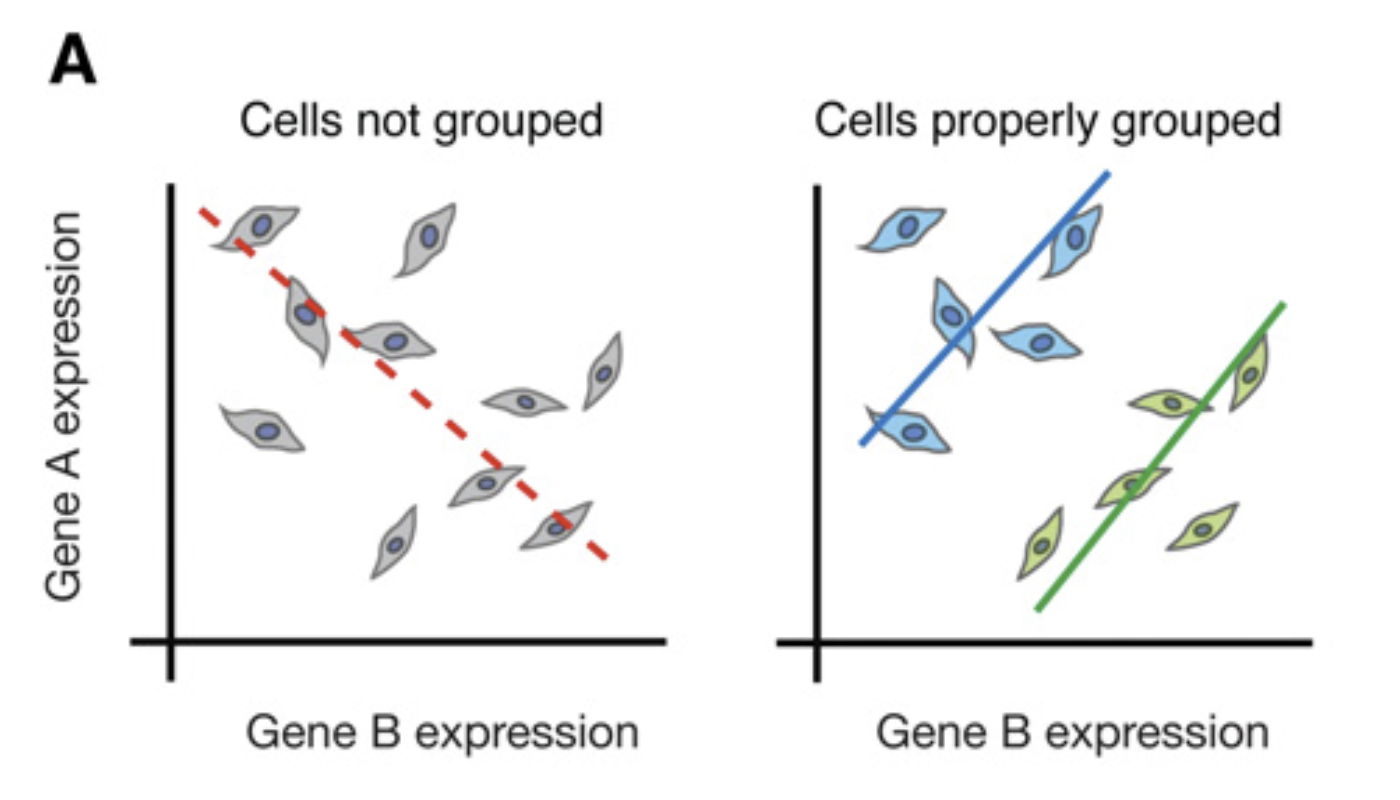
Figure 1.2: In the scRNA-seq analysis, it is important to consider Simpson’s paradox where trends disappear or reverse with different grouping of cells. Image taken from Trapnell (2015).

2. Regulatory vs. Compositional Shifts: Changes in gene expression may reflect either (i) a regulatory change where there is uniform upregulation or downregulation across cells or (ii) a compositional change where there is an enrichment or depletion of specific subpopulations. Careful analysis is required to distinguish between these scenarios, often using compositional modeling or cell-type-specific differential expression methods.

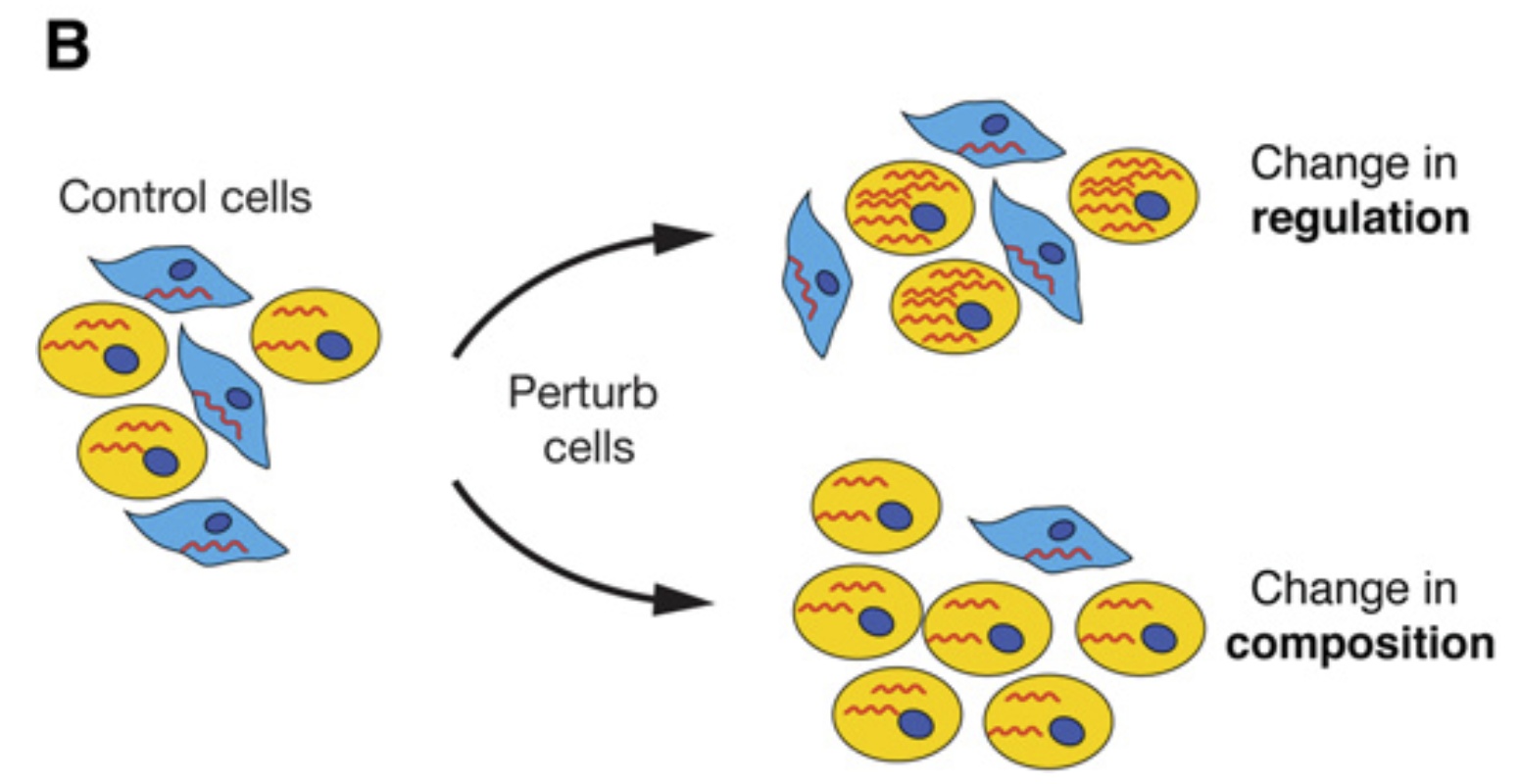
Figure 1.3: Changes in gene expression can be due to a change in regulation or a change in composition. Image taken from Trapnell (2015).

1.2 Experimental Design in scRNA-seq

Before diving into the computational analysis of single-cell datasets, it is worthwhile to understand some of the experimental aspects of scRNA-seq. The choice of experimental technique often have a huge impact on the downstream computational analysis.

1.2.1 Full-length vs. Tag-based RNA-seq

RNA-seq converts RNA into cDNA for sequencing (Section 1.1.1). Two broad strategies exist, namely (i) full-length methods (e.g., Smart-seq2) which capture entire transcripts and is suitable for isoform analysis but biased by transcript length and (ii) tag-based methods (e.g., 10X Genomics) which capture 5’ or 3’ ends of the mRNA molecule and often employ UMIs for accurate quantification but less suitable for isoform analysis.

1.2.2 Unique molecular identifiers (UMI)

Due to the low RNA content in each single cell, PCR-based amplification is often required to generate enough starting material for sequencing. Unique molecular identifier (UMIs) tag cDNA molecules with random barcodes before amplification. Identical UMIs indicate reads from the same original molecule, mitigating PCR amplification bias and enabling molecular quantification (Fig. 1.4). Thus, regardless of the extent of amplification, all the cDNA molecules with the same UMI is treated as a single count.

Figure 1.4: UMIs alleviate the problem of PCR amplifcation bias where different RNA fragments may get amplified at different rates (Islam et al. 2014).

1.2.3 scRNA-seq techniques

Recent advances (e.g., droplet microfluidics) allow for the profiling of millions to hundreds of millions of cells. This “single-cell explosion” is also accelerated by the emergence of commercial kits e.g. from 10X Genomics & Parse Bioscience, allowing for more consistent and higher throughput generation of single-cell libraries.

Figure 1.5: Single-cell explosion in the number of cells being studied (Svensson, Vento-Tormo, and Teichmann 2018).

Key distinctions among scRNA-seq techniques include differences in (i) single-cell capture strategy and (ii) RNA quantification.

For single-cell capture, methods vary from well-based to droplet-based to combinatorial barcoding approaches with increasing number of cells captured in a single library. Well-based methods have isolated single cells placed in individual wells and the well sizes can be miniaturised into microwells to accommodate more cells being captured. Droplet-based approaches encapsulates cells with barcoded particles in water-in-oil droplets while combinatorial barcoding approaches introduces barcodes progressively and relies on the large combinations of barcodes when multiple barcodes are concatenated.

For the quantification of RNA abundance, techniques can be separated into full-length or tag-based methods depending on whether the entire RNA molecule is being captured (Section 1.2.1). Full-length methods allow for isoform quantification while tag-based approaches tend to reduce PCR amplification bias. Furthermore, probe-based methods also exist where DNA or RNA probes that bind to specific target sequences within a cell allow for the capture of specific sets of mRNA e.g., from protein coding genes.

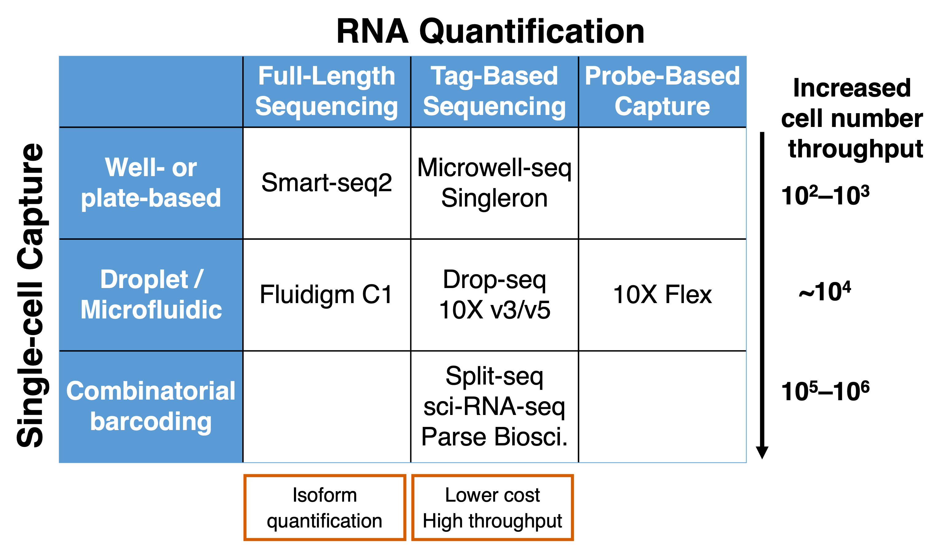
Figure 1.6: scRNA-seq techniques differ in single-cell capture and quantification of RNA abundance.

1.2.4 How many cells to sequence?

The number of cells needed depends on (i) the expected cell states, (ii) the number of cells per cell state and (iii) the detection of rare cell populations.

First, the expected number of cell states is highly dependent on the biology of the system with more diversity requiring more cells and the definition of a cell state. If one is interested in cell subtypes as opposed to major cell types, then the number of cell states of interest increases and more cells would need to be sequenced.

Second, the number of cells per cell state determines the statistical power of downstream analysis. Between full-length and tag-based methods (Section 1.2.3), tag-based methods usually capture less information and thus more cells are required than full-length counterparts. As a rule of thumb, a minimum of 100 and 50 cells per cell state is required for tag-based (e.g. 10X) and full-length methods (e.g. Smart-seq2) respectively. Also, when considering r

Third, regarding rare cell types, more cells would need to be sequence if a desired cell population only comprises a small fraction of the entire sample. The Satija lab has created an online calculator (Fig. 1.7) where users can specify the estimated number of cell states \(m\), the minimum fraction \(p\) and the minimum number of cells per cell state \(n\). The probablity of observing at least \(n\) cells from each cell state is estimated using the negative binomial distribution \(\text{NBcdf}(k; n, p)^m\) where \(k\) is the number of cells in the library i.e. the number of cells to sequence. The calculator then computes the \(k\) required to achieve 95% and 99% probability of observing the rare population.

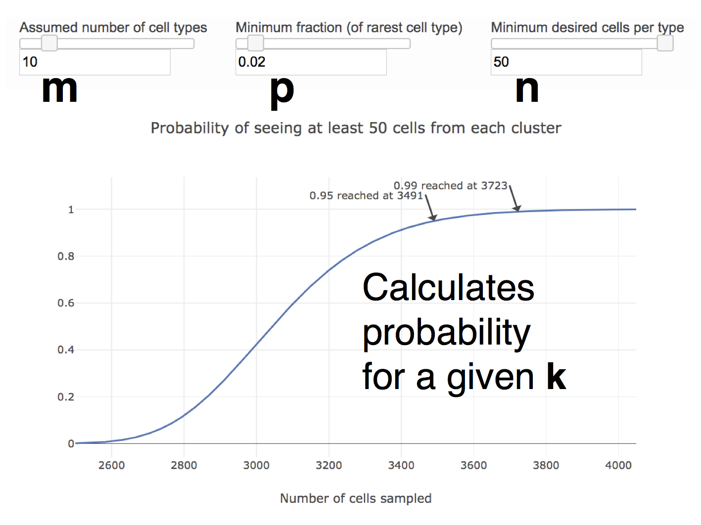
Figure 1.7: Online calculator calculating the number of cells required to have 95% or 99% probability of observing a rare population.

Finally, the intended number of cells to sequence should be amendable to the scRNA-seq technique. For example, 10X v3 kits allow up to 10,000 cells to be captured per channel and a 10X chip comprises 8 such channels. For such droplet-based methods, increasing the number of cells often leads to a higher doublet rate where two or more cells are captured in the same droplet. Such doublets affect downstream analysis and have to be removed bioinformatically. Furthermore, for droplet-based methods, the number of cells loaded initially is not the eventual number of cells that are sequenced. This is because not all the loaded cells will be encapsulated in oil droplets. Current 10X genomics commercial kits (v2 and v3 chemistry) have a capture efficiency of ~60% and these capture efficiencies have to be considered when planning experiments.

1.2.5 Sequencing Depth

Typically, a cell contains approximately \(10^6\) mRNA molecules, which serves as a natural upper bound on the number of reads per cell. However, scRNA-seq techniques are unable to capture all the mRNA and the number of reads per cell is highly technique-dependent. For example, the v2 and v3 10X Genomics commercial kits have a recommended minimum of 50,000 and 20,000 reads per cell respectively while one million reads per cell is common for Smart-seq2 experiments. It is also important to realize that the number of reads does not directly translate to counts in techniques employing UMIs (e.g. 10X). This is because reads with the same UMI are treated as a single molecule / count (Section 1.2.2). From experience, the number of UMIs is often about one eighth to one third (12.5% to 33.3%) of the number of reads for 10X Genomics commercial kits.

Most scRNA-seq techniques generate standard Illumina paired-end constructs, which can then be sequenced using Illumina sequencers. Thus, the choice of sequencer and the number of lanes can be determined after working out the desired number of cells and number of reads per cell.

1.2.6 Batch Effects and Multi-Library Design

In more elaborate studies, not all the cells can be captured in a single library or experiment. Furthermore, multiple libraries might be required to distinguish different samples e.g. different timepoints during a timeseries experiment. When separate single-cell experiments are conducted, batch effects could arise from differences in reagents, operators, or instruments.

To alleviate batch effects, balanced library designs can be employed where samples from the same group e.g. healthy vs disease are in the same batch. For in vitro studies, another way is to introduce a common (and known) population of cells into each single-cell library e.g. introducing embryonic stem cells in a differentiation experiment. In the absence of batch effects, these “overlapping” samples between different batches should cluster together. Also, these common cells can be used to “align” the samples across different batches using computational data integration methods (Section ??).

From the experimental end, experiments are best performed using similar conditions with the same operator. More importantly, one should ensure that sequencing reads are distributed evenly across sequencing lanes as sequencing differences can sometimes introduce significant batch effects. Another strategy is to include multiple samples in a single library and then demultiplex the samples either via genotype or other approaches. Since the multiple samples are within the same library, batch effects should be minimal.

1.2.7 Single-Nucleus RNA-seq (snRNA-seq)

Conventionally, scRNA-seq is performed with intact cells which requires fresh tissue samples or cell cultures. This presents a major roadblock to frozen / fixed samples or tissues that cannot be readily dissociated. To address this, single-nucleus RNA-seq can be performed by capturing only the nuclei instead of whole cells (Habib et al. 2017). Single-nucleus RNA-seq allow for single-cell measurements on frozen samples.

In a recent benchmarking study, Ding et al. (2020) found that single-nucleus RNA-seq generally performed well for sensitivity and classification of cell types. The transcriptome captured via single-cell and single-nucleus approaches are often comparable with some noticeable difference due to the omission of cytoplasmic RNA. In particular, ribosomal and mitochondrial (MT) RNA are no longer present in single-nucleus RNA-seq. This might be beneficial as these ribosomal and MT RNA often take up the majority of reads in scRNA-seq. Furthermore, single-nucleus libraries often contain more intronic reads from unspliced pre-mRNA. This requires a “pre-mRNA” transcriptome reference during the mapping of reads.

1.3 Computational Analysis of scRNA-seq Data

Next, we discuss the different aspects in the computational analysis of single-cell datasets. This include the various steps in the analysis workflow, introduction to integrative single-cell analysis platforms and challenges that can arise in single-cell analysis.

1.3.1 General Workflow

Despite the large number of studies to date, there is no standardized way to analyse single-cell data. This can be attributed to (i) the noisy nature of the data, which often require elaborate quality control and preprocessing steps, (ii) the large number of cells which opens the possibility of new analysis methods that are previously not applicable to bulk RNA-seq and (iii) the large number of computational tools available which complicates standardization. However, there exist several publications that provide guidelines and best practices for single-cell analysis (Section 7.1.3).

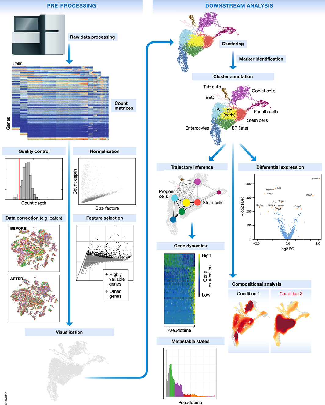
Figure 1.8: Schematic of a typical scRNA-seq analysis workflow. Image taken from Luecken and Theis (2019).

Overall, most single-cell studies converge on a few common steps and a typical analysis pipeline involves:

1. Preprocessing: Alignment, count generation, UMI collapsing (Section ??)

2. Quality control (QC): Filter out low-quality cells/genes (Section ??)

3. Normalization: Adjust for library size and technical noise (Section 2)

4. Feature selection: Identify highly variable genes (HVGs) (Section 2)

5. Dimensionality reduction: PCA, UMAP, or t-SNE (Section 2)

6. Clustering: Identify cell populations and celltype annotation (Section ??)

7. Differential expression (DE): Compare gene expression across clusters (Section ??)

8. Downstream analysis: Trajectory inference, cell-cell interaction, perturbation modeling

1.3.2 Integrated Analysis Platforms

To aid in the analysis of single-cell datasets, there exist several integrative analysis platforms, typically including the above analysis steps from QC to clustering and DE. Some of the widely used analysis platforms include:

• Seurat (R) (Butler et al. 2018): Comprehensive framework which supports multimodal data (e.g., CITE-seq, spatial), which we will be using in this guide

• Scanpy (Python) (Wolf, Angerer, and Theis 2018): Efficient and scalable framework that can work with millions of cells

• Bioconductor ecosystem (R): A series of R-based packages e.g. scater (McCarthy et al. 2017), scran, muscat which are designed to work on SingleCellExperiment or Seurat objects

1.3.3 Challenges in Analysis

Despite the presence of analysis pipelines and numerous analysis tools, several challenges still exist in the computational analysis of single-cell data.

First, scRNA-seq is inherently noisier than its bulk counterpart, owing to the amplification of small amounts of initial RNA material and inadequate sampling in terms of the relatively small number of sequencing reads per single cell. Thus, single-cell data is sparse where most of the gene expression (>80%) are dominated by zero counts. This leads to higher technical variability which has to be accounted for in computational analysis. Notably, it has been shown that the large number of zero values observed in droplet-based scRNA-seq can be still be described using a negative binomial distribution, commonly used to model counts data from bulk RNA-seq (Svensson 2020). This suggest that zero-inflated models which include a zero inflation component to the models are not necessary.

Second, as mentioned in Section 1.2.3, the number of single cells being profiled is increasing at an exponential rate. Thus, computational tools have to be highly scalable and able to work with millions of cells. Ideally, computational tools should have an efficient memory footprint and scale linearly with respect to the number of cells. Consequently, many tools that scale poorly have become disused. On the contrary, this has resulted in the preference of certain classes of algorithms such as k-nearest neighour based methods and the use of graph-based algorithms in cell clustering.

Third, the single-cell field is evolving rapidly, with new algorithms emerging and old algorithms becoming obsolete easily. Furthermore, it is prudent to apply different algorithms for the same analysis task as different tools may have their inherent biases. Thus, it is important to be aware of the latest developments in the field so as to employ the appropriate tools for single-cell analysis.

1.4 Conclusion

Since its inception, scRNA-seq has transformed our understanding of cellular heterogeneity, development, and disease. As the field continues to evolve with innovations in experimental protocols and computational methods, careful design and critical interpretation remain paramount. This section introduces the foundational concepts and up-to-date best practices to help researchers navigate the complexities of single-cell transcriptomics. In the upcoming sections, we will explore the different steps in single-cell data analysis.

References

Adamson, Britt, Thomas M. Norman, Marco Jost, Min Y. Cho, James K. Nuñez, Yuwen Chen, Jacqueline E. Villalta, et al. 2016. “A Multiplexed Single-Cell CRISPR Screening Platform Enables Systematic Dissection of the Unfolded Protein Response.” Cell 167: 1867–82. https://doi.org/10.1016/j.cell.2016.11.048.

Butler, Andrew, Paul Hoffman, Peter Smibert, Efthymia Papalexi, and Rahul Satija. 2018. “Integrating Single-Cell Transcriptomic Data Across Different Conditions, Technologies, and Species.” Nature Biotechnology 36: 411–20. https://doi.org/10.1038/nbt.4096.

Ding, Jiarui, Xian Adiconis, Sean K. Simmons, Monika S. Kowalczyk, Cynthia C. Hession, Nemanja D. Marjanovic, Travis K. Hughes, et al. 2020. “Systematic Comparison of Single-Cell and Single-Nucleus RNA-Sequencing Methods.” Nature Biotechnology. https://doi.org/10.1038/s41587-020-0465-8.

Habib, Naomi, Inbal Avraham-Davidi, Anindita Basu, Tyler Burks, Karthik Shekhar, Matan Hofree, Sourav R Choudhury, et al. 2017. “Massively Parallel Single-Nucleus RNA-Seq with DroNc-Seq.” Nature Methods 14: 955–58. https://doi.org/10.1038/nmeth.4407.

Islam, Saiful, Amit Zeisel, Simon Joost, Gioele La Manno, Pawel Zajac, Maria Kasper, Peter Lonnerberg, and Sten Linnarsson. 2014. “Quantitative Single-Cell RNA-Seq with Unique Molecular Identifiers.” Nature Methods 11: 163–66. https://doi.org/10.1038/nmeth.2772.

Luecken, Malte D, and Fabian J Theis. 2019. “Current Best Practices in Single-Cell RNA-Seq Analysis: A Tutorial.” Molecular Systems Biology 15: e8746. https://doi.org/10.15252/msb.20188746.

McCarthy, Davis J., Kieran R. Campbell, Aaron T. L. Lun, and Quin F. Wills. 2017. “Scater: Pre-Processing, Quality Control, Normalization and Visualization of Single-Cell RNA-Seq Data in R.” Bioinformatics 33: 1179--1186. https://doi.org/10.1093/bioinformatics/btw777.

Replogle, Joseph M., Thomas M. Norman, Albert Xu, Jeffrey A. Hussmann, Jin Chen, J. Zachery Cogan, Elliott J. Meer, et al. 2020. “Combinatorial Single-Cell CRISPR Screens by Direct Guide RNA Capture and Targeted Sequencing.” Nature Biotechnology. https://doi.org/10.1038/s41587-020-0470-y.

Saelens, Wouter, Robrecht Cannoodt, Helena Todorov, and Yvan Saeys. 2019. “A Comparison of Single-Cell Trajectory Inference Methods.” Nature Biotechnology 37: 547–54. https://doi.org/10.1038/s41587-019-0071-9.

Svensson, Valentine. 2020. “Droplet scRNA-Seq Is Not Zero-Inflated.” Nature Biotechnology 38: 147–50. https://doi.org/10.1038/s41587-019-0379-5.

Svensson, Valentine, Roser Vento-Tormo, and Sarah A Teichmann. 2018. “Exponential Scaling of Single-Cell RNA-Seq in the Past Decade.” Nature Protocols 13: 599–604. https://doi.org/10.1038/nprot.2017.149.

The Tabula Muris Consortium. 2018. “Single-Cell Transcriptomics of 20 Mouse Organs Creates a Tabula Muris.” Nature 562: 367–72. https://doi.org/10.1038/s41586-018-0590-4.

Trapnell, Cole. 2015. “Defining Cell Types and States with Single-Cell Genomics.” Genome Research 25: 1491–98. https://doi.org/10.1101/gr.190595.115.

Wolf, F. Alexander, Philipp Angerer, and Fabian J. Theis. 2018. “SCANPY: Large-Scale Single-Cell Gene Expression Data Analysis.” Genome Biology 19: 15. https://doi.org/10.1186/s13059-017-1382-0.