Chapter 4 Uncovering Biological Trajectories
4.1 Dimension reduction DR101
Relavance between DR and trajectories
4.1.1 Local vs. global structure in DR
Flowly vs clumpy projections, former good for trajectories, latter good for atlasing
4.1.2 Recap on PCA, t-SNE and UMAP
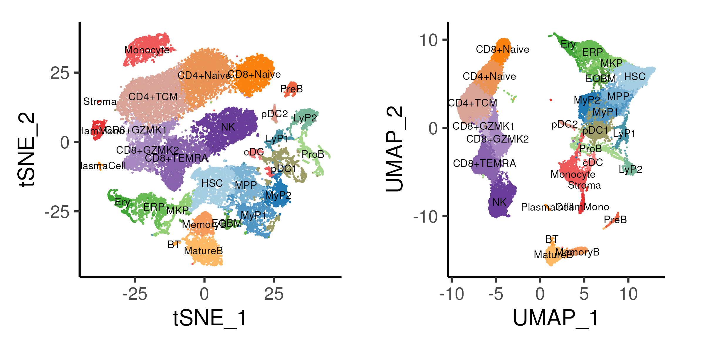
Figure 4.1: t-SNE and UMAP projections of the bone marrow data coloured by cell annotation derived from previous section.
4.1.3 Diffusion maps
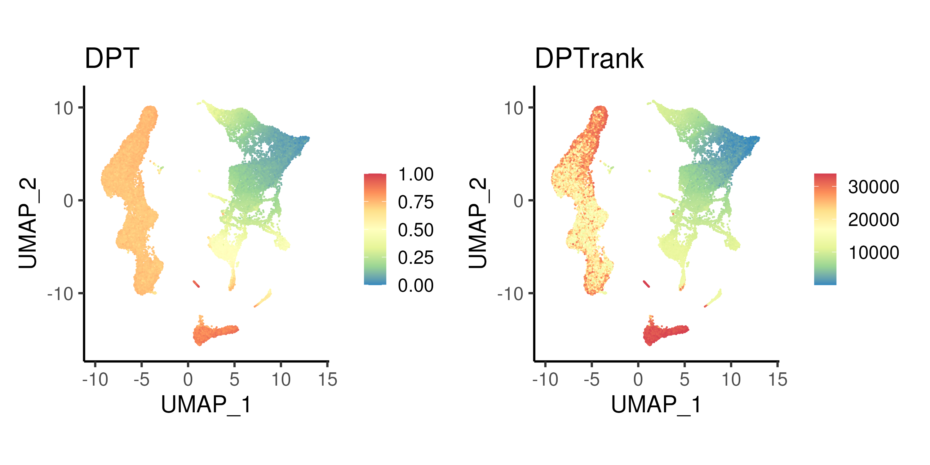
Figure 4.2: Diffusion pseudotime calculated using top 10 DCs and the corresponding rank.
4.1.4 Code
##### Load required packages
rm(list = ls())
library(data.table)
library(Matrix)
library(ggplot2)
library(plotly)
library(patchwork)
library(RColorBrewer)
library(Seurat)
library(reticulate)
library(pdist)
library(phateR)
library(SeuratWrappers)
library(monocle3)
library(slingshot)
library(tradeSeq)
library(pheatmap)
library(clusterProfiler)
library(msigdbr)
library(BiocParallel)
if(!dir.exists("images/")){dir.create("images/")} # Folder to store outputs

### Define color palettes and plot themes
colLib = brewer.pal(7, "Paired")
names(colLib) = c("BM0pos", "BM0neg", "BM7pos", "BM7neg",
                  "BM9pos", "BM9neg", "BM2pos")
colDnr = colLib[c(1,3,5,7)]
names(colDnr) = c("BM0", "BM7", "BM9", "BM2")
colGEX = c("grey85", brewer.pal(7, "Reds"))
colCcy = c("black", "blue", "darkorange")
plotTheme <- theme_classic(base_size = 18)
os <- import("os")
py_run_string("r.os.environ['OMP_NUM_THREADS'] = '4'")
nC <- 4 # Number of threads / cores on computer

### Load stuff from previous script
seu <- readRDS("bmSeu.rds")
nPC <- 23 # determined from elbow plot
nClust <- uniqueN(Idents(seu))         # Setup color palette
colCls <- colorRampPalette(brewer.pal(n = 10, name = "Paired"))(nClust)


##### Sec4: Trajectory Analysis
### A. Alternate dimension reduction
# Setup python anndata for downstream DFL/DiffMap/PAGA
sc <- import("scanpy", convert = FALSE)
ad <- import("anndata", convert = FALSE)
adata <- sc$AnnData(
  X   = np_array(t(GetAssayData(seu)[VariableFeatures(seu),]), dtype="float32"),
  obs = seu@meta.data[, c("library", "celltype")],
  var = data.frame(geneName = VariableFeatures(seu)))
adata$obsm$update(X_pca = Embeddings(seu, "pca"))
adata$obsm$update(X_umap = Embeddings(seu, "umap"))
adata$var_names <- VariableFeatures(seu)
adata$obs_names <- colnames(seu)
sc$pp$neighbors(adata, n_neighbors = as.integer(30), n_pcs = as.integer(nPC))

# FDL
sc$tl$draw_graph(adata, layout = "fa", init_pos = "X_umap")
oupDR <- py_to_r(adata$obsm['X_draw_graph_fa'])
rownames(oupDR) <- colnames(seu)
colnames(oupDR) <- c("FDL_1","FDL_2")
oupDR = oupDR / 10^(floor(log10(diff(range(oupDR))))-1)
seu[["fdl"]] <- CreateDimReducObject(embeddings = oupDR, key = "FDL_",
                                     assay = DefaultAssay(seu))

p1 <- DimPlot(seu, reduction = "umap", pt.size = 0.1, label = TRUE,
              label.size = 3, cols = colCls) + plotTheme + coord_fixed()
p2 <- DimPlot(seu, reduction = "fdl", pt.size = 0.1, label = TRUE,
              label.size = 3, cols = colCls) + plotTheme + coord_fixed()
ggsave(p1 + p2 & theme(legend.position = "none"),
       width = 10, height = 5, filename = "images/dimrdFDL.png")

# DiffMaps + DPT pseudotime
sc$tl$diffmap(adata)
oupDR <- py_to_r(adata$obsm['X_diffmap'])
rownames(oupDR) <- colnames(seu)
colnames(oupDR) <- paste0("DC_", 0:(15-1))
oupDR <- oupDR[, paste0("DC_", seq(10))]
seu[["diffmap"]] = CreateDimReducObject(embeddings = oupDR, key = "DC_",
                                        assay = DefaultAssay(seu))

p3 <- list()
for(i in 2:10){
  p3[[paste0("DC1",i)]] <-
    DimPlot(seu, reduction = "diffmap", pt.size = 0.1, label = TRUE,
            label.size = 3, cols = colCls, dims = c(1,i)) + plotTheme
}
ggsave(wrap_plots(p3) & theme(legend.position = "none"),
       width = 12, height = 12, filename = "images/dimrdDiffmap.png")

# DPT pseudotime
rootCelltype <- "HSC"
oupDR <- py_to_r(adata$obsm['X_diffmap'])
rownames(oupDR) <- colnames(seu)
colnames(oupDR) <- paste0("DC_", 0:(15-1))
oupDR <- oupDR[, paste0("DC_", seq(10))]
oupDR <- data.table(celltype = seu$celltype, oupDR)
tmp <- oupDR[, lapply(.SD, mean), by = "celltype"]    # celltype centroid
tmp <- tmp[celltype != rootCelltype]
tmp <- data.frame(tmp[, -1], row.names = tmp$celltype)
oupDR$sampleID <- colnames(seu)
oupDR <- oupDR[celltype == rootCelltype]
oupDR <- data.frame(oupDR, row.names = oupDR$sampleID)
oupDR <- oupDR[, colnames(tmp)]
tmp <- as.matrix(pdist(oupDR, tmp))
rownames(tmp) <- rownames(oupDR)
iTip <- grep(names(which.max(rowSums(tmp))), colnames(seu))          # tip cell
py_run_string(paste0("r.adata.uns['iroot'] = ", as.integer(iTip-1))) # 0-base
sc$tl$dpt(adata)
seu$DPT <- py_to_r(adata$obs$dpt_pseudotime)
seu$DPTrank <- rank(seu$DPT)
# seu$tmp = seu$celltype; seu$tmp[iTip] = NA; seu$tmp2=0.1; seu$tmp2[iTip]=3
# DimPlot(seu, reduction = "umap", pt.size = seu$tmp2, group.by = "tmp")

p1 <- FeaturePlot(seu, reduction = "umap", pt.size = 0.1, feature = "DPT") +
  scale_color_distiller(palette = "Spectral") + plotTheme + coord_fixed()
p2 <- FeaturePlot(seu, reduction = "umap", pt.size = 0.1, feature = "DPTrank") +
  scale_color_distiller(palette = "Spectral") + plotTheme + coord_fixed()
ggsave(p1 + p2 + plot_layout(ncol = 2),
       width = 10, height = 5, filename = "images/dimrdDPT.png")

# PHATE
oupPhate = phate(t(GetAssayData(seu)[VariableFeatures(seu), ]),
                 knn = 30, npca = nPC, seed = 0)
oupDR = oupPhate$embedding
oupDR = oupDR / 10^(floor(log10(diff(range(oupDR)))))
rownames(oupDR) = colnames(seu)
colnames(oupDR) = c("PHATE_1","PHATE_2")
seu[["phate"]] <- CreateDimReducObject(embeddings = oupDR, key = "PHATE_",
                                       assay = DefaultAssay(seu))

p1 <- DimPlot(seu, reduction = "umap", pt.size = 0.1, label = TRUE,
              label.size = 3, cols = colCls) + plotTheme + coord_fixed()
p2 <- DimPlot(seu, reduction = "phate", pt.size = 0.1, label = TRUE,
              label.size = 3, cols = colCls) + plotTheme + coord_fixed()
ggsave(p1 + p2 & theme(legend.position = "none"),
       width = 10, height = 5, filename = "images/dimrdPHATE.png")

# 3D UMAP
seu <- RunUMAP(seu, dims = 1:nPC, n.components = 3,
               reduction.name = "umap3d", reduction.key = "UMAP3D_")
ggData <- data.table(seu@reductions$umap3d@cell.embeddings)
ggData$celltype <- seu$celltype
fwrite(ggData, sep = "\t", file = "images/dimrd3dumap.txt.gz")
p1 <- plot_ly(ggData, x = ~UMAP3D_1, y = ~UMAP3D_2, z = ~UMAP3D_3,
              color = ~celltype, type = "scatter3d", size = 1, colors = colCls)
htmlwidgets::saveWidget(partial_bundle(p1), file = "images/dimrd3dumap.html",
                        selfcontained = TRUE)
4.2 Trajectory inference and pseudotime
4.2.3 Different trajectory inference methods
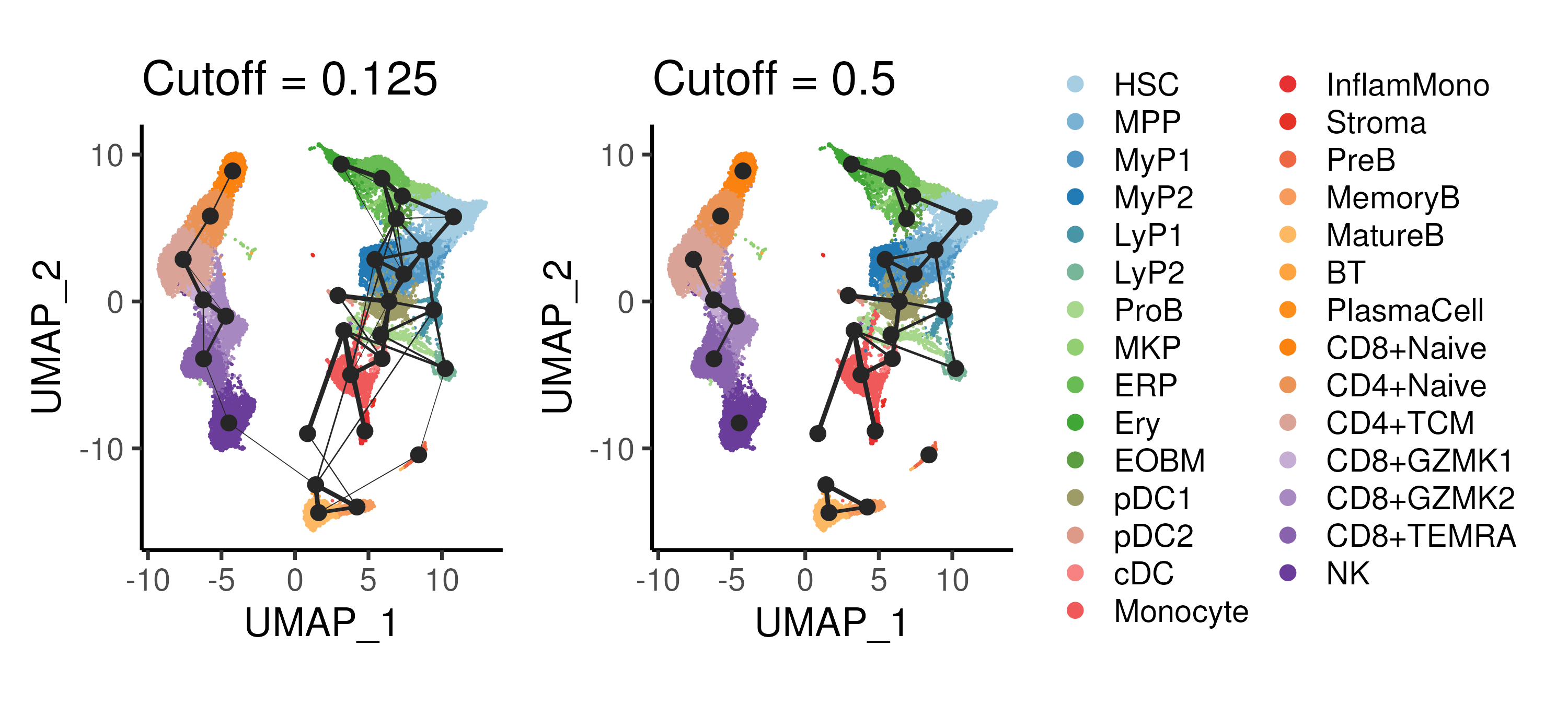
Figure 4.3: PAGA inference of cluster-cluster relationships in the bone marrow data with different cutoffs applied to the cluster connectivity.
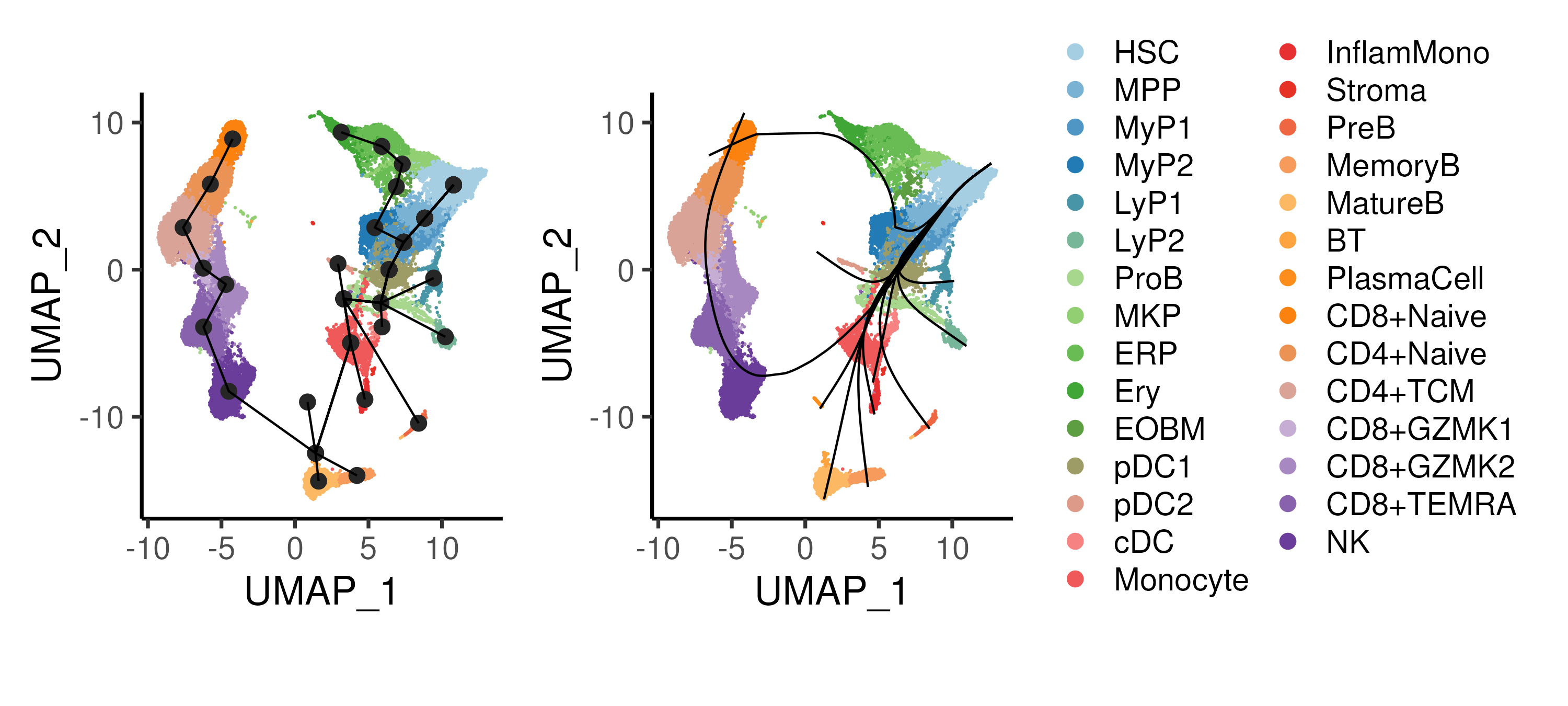
Figure 4.4: Trajectory inference using the Slingshot algorithm, showing the cluster connectivity and smoothed trajectories. Cells are coloured by annotated cell types.
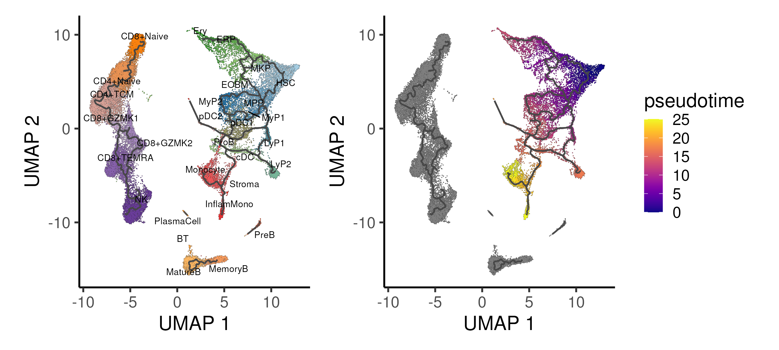
Figure 4.5: Trajectory inference using the Monocle algorithm applied onto the UMAP space, showing the different trajectories and inferred pseudotime for the CD34 progenitor “island”. Cells are coloured by annotated cell types.
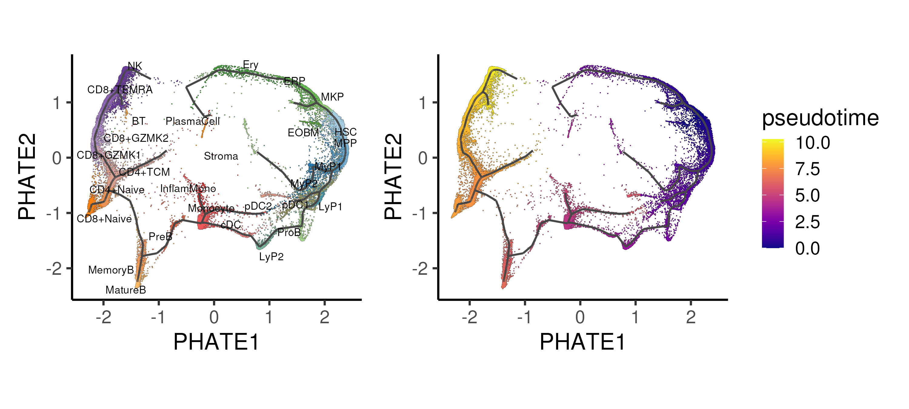
Figure 4.6: Trajectory inference using the Monocle algorithm applied onto the PHATE space, showing the different trajectories and inferred pseudotime for the CD34 progenitor “island”. Cells are coloured by annotated cell types.
4.2.4 Code
### B. Trajectory inference
# PAGA
sc$tl$paga(adata, groups = "celltype")
oupPAGA <- py_to_r(adata$uns[["paga"]]$connectivities$todense())
oupPAGA[upper.tri(oupPAGA)] <- 0
oupPAGA <- data.table(source = levels(seu$celltype), oupPAGA)
colnames(oupPAGA) <- c("source", levels(seu$celltype))
oupPAGA <- melt.data.table(oupPAGA, id.vars = "source",
                           variable.name = "target", value.name = "weight")
seu@misc$PAGA <- oupPAGA     # Store PAGA results into Seurat object

ggData = data.table(celltype = seu$celltype, seu@reductions$umap@cell.embeddings)
ggData = ggData[,.(UMAP_1 = mean(UMAP_1), UMAP_2 = mean(UMAP_2)), by = "celltype"]
oupPAGA = ggData[oupPAGA, on = c("celltype" = "source")]
oupPAGA = ggData[oupPAGA, on = c("celltype" = "target")]
colnames(oupPAGA) = c("celltypeA","UMAP1A","UMAP2A","celltypeB",
                                  "UMAP1B","UMAP2B","weight")
oupPAGA$plotWeight = oupPAGA$weight * 1

p3 <- DimPlot(seu, reduction = "umap", pt.size = 0.1, label = FALSE,
              label.size = 3, cols = colCls) + plotTheme + coord_fixed()
p1 <- p3 +
  geom_point(data = ggData, aes(UMAP_1, UMAP_2), size = 3, color = "grey15") +
  geom_segment(data = oupPAGA[weight > 0.125], color = "grey15",
               linewidth = oupPAGA[weight > 0.125]$plotWeight,
               aes(x = UMAP1A, y = UMAP2A, xend = UMAP1B, yend = UMAP2B)) +
  ggtitle("Cutoff = 0.125")
p2 <- p3 +
  geom_point(data = ggData, aes(UMAP_1, UMAP_2), size = 3, color = "grey15") +
  geom_segment(data = oupPAGA[weight > 0.5], color = "grey15",
               linewidth = oupPAGA[weight > 0.5]$plotWeight,
               aes(x = UMAP1A, y = UMAP2A, xend = UMAP1B, yend = UMAP2B)) +
  ggtitle("Cutoff = 0.5")
ggsave(p1 + p2 + plot_layout(guides = "collect"),
       width = 10, height = 4.5, filename = "images/dimrdTrajPAGA.png")

# Slingshot
sce <- as.SingleCellExperiment(seu)
sce <- slingshot(sce, reducedDim = 'UMAP', clusterLabels = sce$celltype,
                 start.clus = 'HSC', approx_points = 200)

slsMST <- slingMST(sce, as.df = TRUE)
slsCrv <- slingCurves(sce, as.df = TRUE)
p3 <- DimPlot(seu, reduction = "umap", pt.size = 0.1, label = FALSE,
              label.size = 3, cols = colCls) + plotTheme + coord_fixed()
p1 <- p3 +
  geom_point(data = slsMST, aes(UMAP_1, UMAP_2), size = 3, color = "grey15") +
  geom_path(data = slsMST %>% arrange(Order),
            aes(UMAP_1, UMAP_2, group = Lineage))
p2 <- p3 +
  geom_path(data = slsCrv %>% arrange(Order),
            aes(UMAP_1, UMAP_2, group = Lineage))
ggsave(p1 + p2 + plot_layout(guides = "collect"),
       width = 10, height = 4.5, filename = "images/dimrdTrajSlingshot.png")

# Monocle on UMAP
cds <- as.cell_data_set(seu)
cds <- cluster_cells(cds, reduction_method = "UMAP")
cds <- learn_graph(cds)
cds <- order_cells(cds, root_cells = colnames(cds)[iTip])

p1 <- plot_cells(
  cds, color_cells_by = "celltype",
  label_groups_by_cluster = F, label_branch_points = F, label_roots = F,
  label_leaves = F, cell_size = 0.2, group_label_size = 3) +
  scale_color_manual(values = colCls) + plotTheme + coord_fixed() +
  theme(legend.position = "none")
p2 <- plot_cells(
  cds, color_cells_by = "pseudotime",
  label_groups_by_cluster = F, label_branch_points = F, label_roots = F,
  label_leaves = F, cell_size = 0.2) + plotTheme + coord_fixed()
ggsave(p1 + p2,
       width = 10, height = 4.5, filename = "images/dimrdTrajMono.png")

# Monocle on PHATE
cds2 <- as.cell_data_set(seu)
cds2@int_colData@listData[["reducedDims"]]@listData[["UMAP"]] <-
  cds2@int_colData@listData[["reducedDims"]]@listData[["PHATE"]]
cds2 <- cluster_cells(cds2, reduction_method = "UMAP")
cds2 <- learn_graph(cds2)
cds2 <- order_cells(cds2, root_cells = colnames(cds2)[iTip])

p1 <- plot_cells(
  cds2, color_cells_by = "celltype",
  label_groups_by_cluster = F, label_branch_points = F, label_roots = F,
  label_leaves = F, cell_size = 0.2, group_label_size = 3) +
  scale_color_manual(values = colCls) + plotTheme + coord_fixed() +
  theme(legend.position = "none")
p2 <- plot_cells(
  cds2, color_cells_by = "pseudotime",
  label_groups_by_cluster = F, label_branch_points = F, label_roots = F,
  label_leaves = F, cell_size = 0.2) + plotTheme + coord_fixed()
ggsave(p1 + p2 & xlab("PHATE1") & ylab("PHATE2"),
       width = 10, height = 4.5, filename = "images/dimrdTrajMonoPH.png")
4.3 Differential expression in trajectories
4.3.3 Followup Analysis
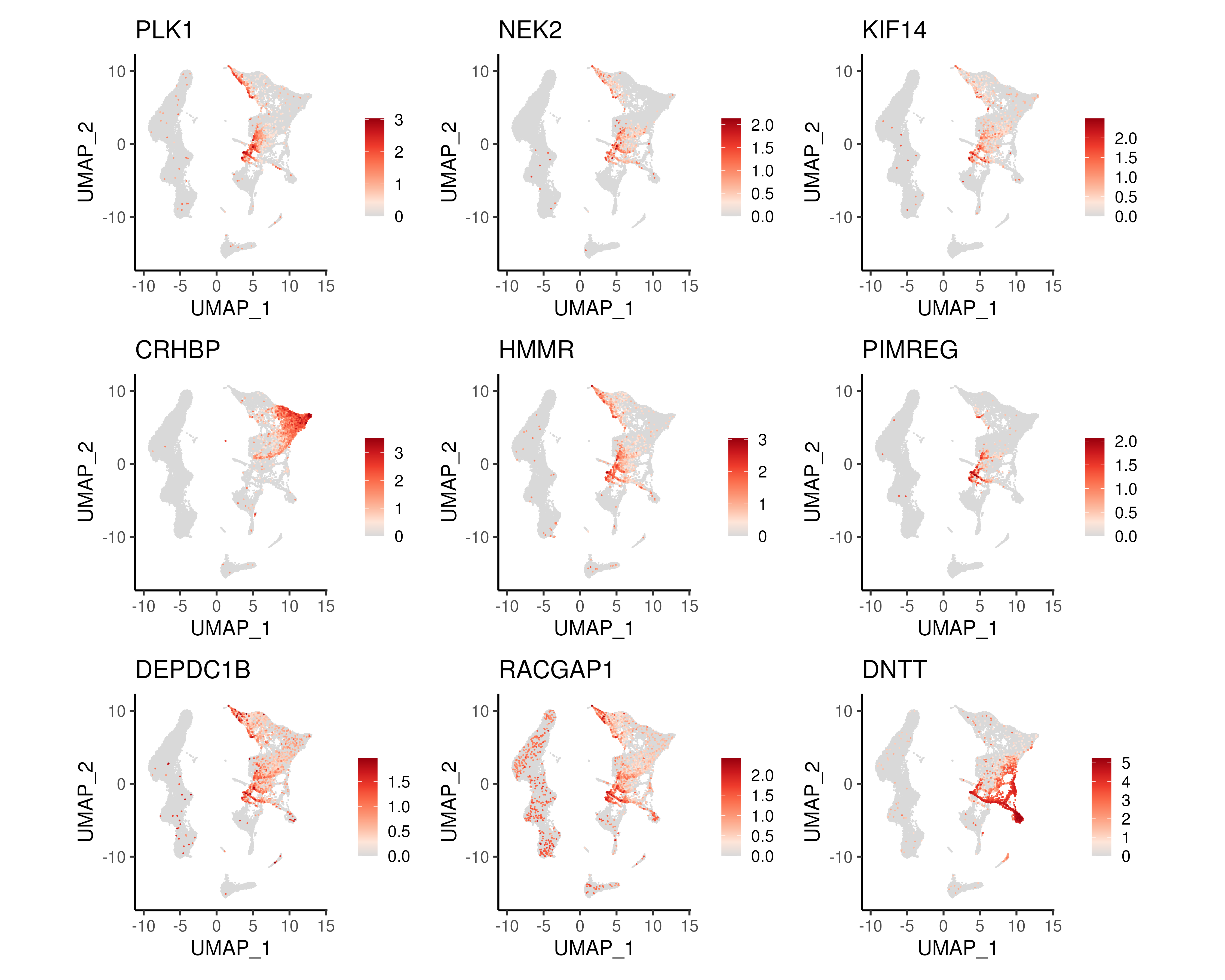
Figure 4.7: UMAP of top 9 DEGs along the HSC->MyP and HSC->LyP trajectories.
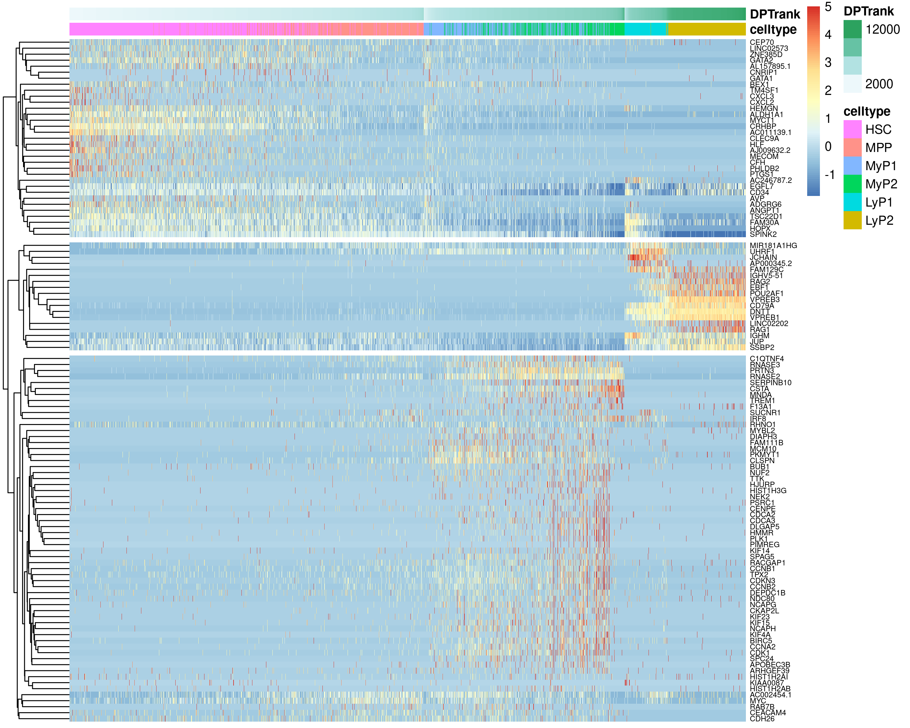
Figure 4.8: Heatmap showing gene expression changes across pseudotime for the top genes changing along the HSC->MyP and HSC->LyP trajectories.
4.3.4 Code
### C. DE on trajectories
# Focus on two lineage:
### HSC -> MPP -> MyP1 -> MyP2
### HSC -> MPP -> LyP1 -> LyP2
# Trade-seq setup
set.seed(42)
inpCells <- c("HSC","MPP","MyP1","MyP2","LyP1","LyP2")
inpCells <- seu@meta.data[seu$celltype %in% inpCells, ]
inpCells <- data.table(cell = rownames(inpCells), inpCells)
inpCells$segment <- "Common"
inpCells[celltype %in% c("MyP1","MyP2")]$segment <- "Myeloid"
inpCells[celltype %in% c("LyP1","LyP2")]$segment <- "Lymphoid"
inpCells$segment <- factor(inpCells$segment,
                           levels = c("Common", "Myeloid", "Lymphoid"))

inpCts <- GetAssayData(object = seu, slot = "counts")[, inpCells$cell]
inpCts <- inpCts[rowSums(inpCts >= 3) >= 20, ] # Relax this if you want more genes
inpDPT <- cbind(inpCells$DPT, inpCells$DPT)
rownames(inpDPT) <- inpCells$cell
colnames(inpDPT) <- c("Myeloid", "Lymphoid")
inpWgt <- matrix(data = 0, nrow = nrow(inpCells), ncol = 2)
rownames(inpWgt) <- inpCells$cell
colnames(inpWgt) <- c("Myeloid", "Lymphoid")
inpWgt[inpCells$celltype %in% c("HSC","MPP"), 1:2] <- 1/2
inpWgt[inpCells$celltype %in% c("MyP1","MyP2"), 1] <- 1
inpWgt[inpCells$celltype %in% c("LyP1","LyP2"), 2] <- 1

# Actual trade-seq run
register(MulticoreParam(30))
oupTrSK <- evaluateK(counts = inpCts, pseudotime = inpDPT, cellWeights = inpWgt,
                     nGenes = 250)
dev.copy(png, width = 8, height = 6, units = "in", res = 300,
         filename = "images/dimrdTrajDEk.png"); dev.off()
oupTrS <- fitGAM(counts = inpCts, pseudotime = inpDPT, cellWeights = inpWgt,
                 nknots = 7)

# Association test
oupTrSres1 <- associationTest(oupTrS, lineages = TRUE)
oupTrSres1 <- data.table(gene = rownames(oupTrSres1), oupTrSres1)
oupTrSres1$padj_all <- p.adjust(oupTrSres1$pvalue, method = "fdr")
oupTrSres1$padj_1 <- p.adjust(oupTrSres1$pvalue_1, method = "fdr")
oupTrSres1$padj_2 <- p.adjust(oupTrSres1$pvalue_2, method = "fdr")
oupTrSres1 <- oupTrSres1[order(-meanLogFC)]

p1 <- FeaturePlot(seu, reduction = "umap", pt.size = 0.1, order = TRUE,
            feature = oupTrSres1[order(-meanLogFC)]$gene[1:9]) &
  scale_color_gradientn(colors = colGEX) & plotTheme & coord_fixed()
ggsave(p1, width = 15, height = 12, filename = "images/dimrdTrajDEassoc.png")

ggData <- GetAssayData(object = seu, slot = "data")
ggData <- ggData[oupTrSres1[meanLogFC > 5]$gene,
                 inpCells[order(segment, DPT)]$cell]
ggData <- t(scale(t(ggData)))
ggData[ggData > 5] <- 5; ggData[ggData < -5] <- -5
tmp <- data.frame(celltype = inpCells$celltype,
                  DPTrank = inpCells$DPTrank,
                  row.names = inpCells$cell)
pheatmap(as.matrix(ggData), cluster_cols = FALSE, show_colnames = FALSE,
         cutree_rows = 3, gaps_col = cumsum(table(tmp$segment)),
         annotation_col = tmp, fontsize_row = 6,
         width = 10, height = 8,
         filename = "images/dimrdTrajDEassocH.png")